10wk-1: 중간고사

Author

최규빈

Published

May 8, 2023

제출은 *.ipynb, *.html, *.pdf 파일로 제출할 것

ipynb 파일형태제출을 권장함.

Imports

import pandas as pd
import numpy as np
import matplotlib.pyplot as plt
import yfinance as yf
import PIL
import io 
import requests

1. Numpy and Pandas (35점)

FIFA23

(1)--(3) 아래는 FIFA23 자료를 불러오는 코드이다.

df=pd.read_csv('https://raw.githubusercontent.com/guebin/DV2022/master/posts/FIFA23_official_data.csv').drop(columns=['Loaned From', 'Best Overall Rating']).dropna().reset_index(drop=True)
df.head()

	ID	Name	Age	Photo	Nationality	Flag	Overall	Potential	Club	Club Logo	...	Work Rate	Body Type	Real Face	Position	Joined	Contract Valid Until	Height	Weight	Release Clause	Kit Number
0	209658	L. Goretzka	27	https://cdn.sofifa.net/players/209/658/23_60.png	Germany	https://cdn.sofifa.net/flags/de.png	87	88	FC Bayern München	https://cdn.sofifa.net/teams/21/30.png	...	High/ Medium	Unique	Yes	<span class="pos pos28">SUB	Jul 1, 2018	2026	189cm	82kg	€157M	8.0
1	212198	Bruno Fernandes	27	https://cdn.sofifa.net/players/212/198/23_60.png	Portugal	https://cdn.sofifa.net/flags/pt.png	86	87	Manchester United	https://cdn.sofifa.net/teams/11/30.png	...	High/ High	Unique	Yes	<span class="pos pos15">LCM	Jan 30, 2020	2026	179cm	69kg	€155M	8.0
2	224334	M. Acuña	30	https://cdn.sofifa.net/players/224/334/23_60.png	Argentina	https://cdn.sofifa.net/flags/ar.png	85	85	Sevilla FC	https://cdn.sofifa.net/teams/481/30.png	...	High/ High	Stocky (170-185)	No	<span class="pos pos7">LB	Sep 14, 2020	2024	172cm	69kg	€97.7M	19.0
3	192985	K. De Bruyne	31	https://cdn.sofifa.net/players/192/985/23_60.png	Belgium	https://cdn.sofifa.net/flags/be.png	91	91	Manchester City	https://cdn.sofifa.net/teams/10/30.png	...	High/ High	Unique	Yes	<span class="pos pos13">RCM	Aug 30, 2015	2025	181cm	70kg	€198.9M	17.0
4	224232	N. Barella	25	https://cdn.sofifa.net/players/224/232/23_60.png	Italy	https://cdn.sofifa.net/flags/it.png	86	89	Inter	https://cdn.sofifa.net/teams/44/30.png	...	High/ High	Normal (170-)	Yes	<span class="pos pos13">RCM	Sep 1, 2020	2026	172cm	68kg	€154.4M	23.0

5 rows × 27 columns

(1) 공백이 포함된 column이름이 총 몇개인지 count하는 코드를 작성하라.

hint 모두 11개의 column name에 공백이 포함되어있음

(풀이)

sum([' ' in name for name in df.columns])

(2) column name에 공백이 포함된 열을 출력하라.

(풀이)

df.loc[:,[' ' in name for name in df.columns]]

	Club Logo	Preferred Foot	International Reputation	Weak Foot	Skill Moves	Work Rate	Body Type	Real Face	Contract Valid Until	Release Clause	Kit Number
0	https://cdn.sofifa.net/teams/21/30.png	Right	4.0	4.0	3.0	High/ Medium	Unique	Yes	2026	€157M	8.0
1	https://cdn.sofifa.net/teams/11/30.png	Right	3.0	3.0	4.0	High/ High	Unique	Yes	2026	€155M	8.0
2	https://cdn.sofifa.net/teams/481/30.png	Left	2.0	3.0	3.0	High/ High	Stocky (170-185)	No	2024	€97.7M	19.0
3	https://cdn.sofifa.net/teams/10/30.png	Right	4.0	5.0	4.0	High/ High	Unique	Yes	2025	€198.9M	17.0
4	https://cdn.sofifa.net/teams/44/30.png	Right	3.0	3.0	3.0	High/ High	Normal (170-)	Yes	2026	€154.4M	23.0
...	...	...	...	...	...	...	...	...	...	...	...
16359	https://cdn.sofifa.net/teams/114628/30.png	Right	1.0	3.0	1.0	Medium/ Medium	Normal (185+)	No	2027	€218K	35.0
16360	https://cdn.sofifa.net/teams/1478/30.png	Right	1.0	2.0	1.0	Medium/ Medium	Lean (185+)	No	2026	€188K	21.0
16361	https://cdn.sofifa.net/teams/113796/30.png	Right	1.0	2.0	1.0	Medium/ Medium	Lean (185+)	No	2023	€142K	12.0
16362	https://cdn.sofifa.net/teams/112260/30.png	Right	1.0	2.0	1.0	Medium/ Medium	Normal (185+)	No	2021	€214K	40.0
16363	https://cdn.sofifa.net/teams/702/30.png	Left	1.0	2.0	1.0	Medium/ Medium	Normal (185+)	No	2021	€131K	30.0

16364 rows × 11 columns

(3) 데이터프레임을 올바르게 해석한 사람을 모두 고르시오 (모두 맞출경우만 정답으로 인정)

세민: 데이터프레임에는 모두 27개의 열이 있다.
성재: 한국선수(Nationality==Korea Republic)와 일본선수(Nationality==Japan)의 Overall의 평균값은 일본이 더 높다.
민정: 총 159개의 나라선수들이 포함되어 있다.
슬기: 선수들의 연령이 25세이상(>=)인 선수들은 그렇지 않은 선수들보다 평균적으로 키(Height)가크다.

(풀이)

세민: 데이터프레임에는 모두 27개의 열이 있다 -> True

len(df.columns) == 27

True

성재: 한국선수(Nationality==Korea Republic)와 일본선수(Nationality==Japan)의 Overall의 평균값은 일본이 더 높다. -> True

df.query('Nationality == "Korea Republic"').Overall.mean() < df.query('Nationality == "Japan"').Overall.mean()

True

민정: 총 159개의 나라선수들이 포함되어 있다. -> True

len(set(df.Nationality))==159

True

슬기: 선수들의 연령이 25세이상(>=)인 선수들은 그렇지 않은 선수들보다 평균적으로 키(Height)가크다. -> True

_old = np.mean([int(height[:3]) for height in df.query('Age>=25').Height.tolist()]) 
_young =  np.mean([int(height[:3]) for height in df.query('Age<25').Height.tolist()]) 
_old > _young

True

삼성전자의 주가

(4)--(5) 다음은 삼성전자의 주가를 크롤링하는 코드이다.

start_date = "2023-01-01"
end_date = "2023-05-02"
y = yf.download("005930.KS", start=start_date, end=end_date)['Adj Close'].to_numpy()

[*********************100%***********************]  1 of 1 completed

삼성전자의 주가 \({\boldsymbol y}\)를 시각화하면 아래와 같다.

plt.plot(y)

(4) 아래와 같은 변환을 이용하여 \({\boldsymbol y}\)를 \(\tilde {\boldsymbol y}\)로 변환하고 결과를 시각화하라.

\(\tilde{y}_1= \frac{1}{4}(3y_1 + y_2)\)
\(\tilde{y}_i= \frac{1}{4}(y_{i-1}+2y_i+y_{i+1})\), for \(i=2,3,\dots,n-1\)
\(\tilde{y}_n= \frac{1}{4}(y_{n-1}+3y_{n})\)

hint: 아래의 코드를 관찰

np.eye(4) + np.array([abs(i-j)<2 for i in range(4) for j in range(4)]).reshape(4,4)

array([[2., 1., 0., 0.],
       [1., 2., 1., 0.],
       [0., 1., 2., 1.],
       [0., 0., 1., 2.]])

(풀이)

T = len(y)
M = (np.eye(T) + np.array([abs(i-j)<2 for i in range(T) for j in range(T)]).reshape(T,T))/4
M[0,0] = 3/4; M[-1,-1]= 3/4 
plt.plot(y,label=r'$y$')
plt.plot(M@y,'--',label=r'$M@y$')
plt.legend()

<matplotlib.legend.Legend at 0x7f6efc12bb80>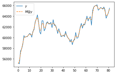

(5) (4)의 변환을 50회 반복적용하고 결과를 시각화하라.

plt.plot(y,label=r'$y$')
plt.plot(np.linalg.matrix_power(M,50)@y,'--',label=r'$M^{50}@y$')
plt.legend()

<matplotlib.legend.Legend at 0x7f6efc6694f0>

회귀모형

(6)--(7) \((x_i,y_i)\)가 아래와 같이 주어졌다고 가정하자.

x =  np.array([0.00983, 0.01098, 0.02951, 0.0384 , 0.03973, 0.04178, 0.0533 ,
               0.058  , 0.09454, 0.1103 , 0.1328 , 0.1412 , 0.1497 , 0.1664 ,
               0.1906 , 0.1923 , 0.198  , 0.2141 , 0.2393 , 0.2433 , 0.3157 ,
               0.3228 , 0.3418 , 0.3552 , 0.3918 , 0.3962 , 0.4    , 0.4482 ,
               0.496  , 0.507  , 0.53   , 0.5654 , 0.582  , 0.5854 , 0.5854 ,
               0.6606 , 0.7007 , 0.723  , 0.7305 , 0.7383 , 0.7656 , 0.7725 ,
               0.831  , 0.8896 , 0.9053 , 0.914  , 0.949  , 0.952  , 0.9727 ,
               0.982  ])
y =  np.array([0.7381, 0.7043, 0.3937, 0.1365, 0.3784, 0.3028, 0.1037, 0.3846,
               0.706 , 0.7572, 0.2421, 0.232 , 0.9855, 1.162 , 0.4653, 0.6791,
               0.6905, 0.6865, 0.9757, 0.7665, 0.9522, 0.4641, 0.5498, 1.1509,
               0.5288, 1.1195, 1.1659, 1.4341, 1.2779, 1.1648, 1.4002, 0.7472,
               0.9142, 0.9658, 1.0707, 1.4501, 1.6758, 0.8778, 1.3384, 0.7476,
               1.3086, 1.7537, 1.5559, 1.2928, 1.3832, 1.3115, 1.3382, 1.536 ,           
               1.9177, 1.2069])

plt.plot(x,y,'o')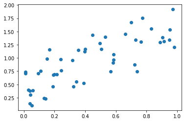

6. 아래의 수식을 이용하여 적절한 추세선 \(\hat{y}_i= \hat{\beta}_0 +\hat{\beta}_1 x_i\)를 구하고 시각화하라.

\[\begin{bmatrix} \hat{\beta}_0 \\ \hat{\beta}_1 \end{bmatrix} = ({\bf X}^T {\bf X})^{-1}{\bf X}^T {\boldsymbol y}, \quad {\bf X}=\begin{bmatrix} 1 & x_1 \\ 1 & x_2 \\ \dots \\ 1 & x_n \end{bmatrix}\]

(풀이)

n = len(x)
X = np.stack([np.ones(n),x],axis=1)
b,a = np.linalg.inv(X.T@X)@X.T@y 
yhat = b+a*x 
plt.plot(x,y,'o')
plt.plot(x,yhat,'--')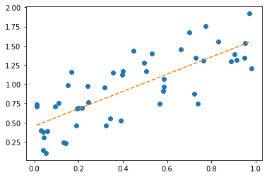

7. \(\frac{1}{n}\sum_{i=1}^{n}(y_i-\hat{y}_i)^2\)을 계산하라.

(풀이)

np.mean((y-yhat)**2)

0.07602899763337416

2. fashion MNIST data (60점)

아래는 9가지의 의류이미지가 저장된 이미지데이터를 불러오는 코드이다.

df_train=pd.read_csv('https://media.githubusercontent.com/media/guebin/PP2023/main/posts/fashion-mnist_train.csv')
df_test=pd.read_csv('https://media.githubusercontent.com/media/guebin/PP2023/main/posts/fashion-mnist_test.csv')

def rshp(row):
    return row.reshape(28,28)

xtrain = np.apply_along_axis(rshp,axis=1,arr=np.array(df_train.iloc[:,1:]))
xtest  = np.apply_along_axis(rshp,axis=1,arr=np.array(df_test.iloc[:,1:]))
ytrain = np.array(df_train.label)
ytest  = np.array(df_test.label)

아래는 데이터에 대한 설명이다.

전체의 이미지의 수는 70000개이며, 60000개의 이미지 \({\tt xtrain}\)에 10000개의 이미지는 \({\tt xtest}\)에 저장되어 있다.
이미지에 대한 라벨은 각각 \({\tt ytrain}\)과 \(\tt ytest\)에 저장되어 있다. 따라서 \(\tt ytrain\)에는 60000개의 이미지에 해당하는 라벨이, \(\tt ytest\)에는 10000개의 이미지에 해당하는 라벨이 기록되어 있다.
보통 분석에서는 60000개의 이미지를 가지고 라벨을 맞추는 “훈련”을 하고 (\({\tt xtrain}\)을 이용하여 \({\tt ytrain}\)을 맞추는 방법을 학습하고), 그러한 훈련이 잘 되었는지 10000개의 이미지를 이용하여 “테스트”한다.
위와 같은 의미로 \(({\tt xtrain}, {\tt ytrain})\) 을 training data set, \(({\tt xtest},{\tt ytest})\) 를 test data set 이라고 부른다. (ref: 위키참고)

아래는 이미지자료와 시각화에 대한 설명이다.

각 이미지는 (28,28) 픽셀의 흑백이미지이다. 따라서 각 이미지는 (28,28,3) 이 아니라 (28,28) 의 shape을 가진 텐서로 구성되어있다.
흑백이미지를 시각화 하기 위해서는 plt.imshow(img, cmap='gray')를 이용한다. 여기에서 \({\tt img}\)은 임의의 2차원 텐서이며 이 예제의 경우 (28,28)의 shape을 가진다.

아래는 \({\tt xtrain}\)의 두번째 이미지, 즉 \({\tt xtrain[1,:,:]}\)를 확인하는 코드의 예시이다.

# plt.imshow(xtrain[1,:,:],cmap='gray')
plt.imshow(xtrain[1],cmap='gray') ## 같은코드임

<matplotlib.image.AxesImage at 0x7f6efb174730>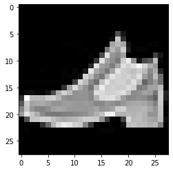

이 이미지에 대한 label은 \({\tt ytrain[1]}\)의 값으로 확인가능하다.

ytrain[1]

이미지와 라벨을 한번에 표현하는 코드는 아래와 같이 작성가능하다.

plt.imshow(xtrain[1],cmap='gray')
plt.title('label={}'.format(ytrain[1]));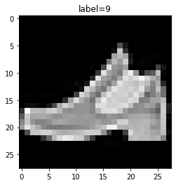

여기에서 9가 의미하는 것은 ’Ankel boot’이며, 다른 숫자가 의미하는 것은 각각 아래와 같다.

labels= {0:'T-shirt/top', 
         1:'Trouser', 
         2:'Pullover', 
         3:'Dress', 
         4:'Coat', 
         5:'Sandal', 
         6:'Shirt', 
         7:'Sneaker', 
         8:'Bag', 
         9:'Ankel boot'}

아래는 \({\tt xtrain}\)의 처음 10개의 이미지를 라벨과 함께 출력하는 코드이다.

fig, ax = plt.subplots(2,5,figsize=(10,5))

ax[0][0].imshow(xtrain[0],cmap='gray'); ax[0][0].set_title('label={}'.format(labels[ytest[0]]));
ax[0][1].imshow(xtrain[1],cmap='gray'); ax[0][1].set_title('label={}'.format(labels[ytest[1]]));
ax[0][2].imshow(xtrain[2],cmap='gray'); ax[0][2].set_title('label={}'.format(labels[ytest[2]]));
ax[0][3].imshow(xtrain[3],cmap='gray'); ax[0][3].set_title('label={}'.format(labels[ytest[3]]));
ax[0][4].imshow(xtrain[4],cmap='gray'); ax[0][4].set_title('label={}'.format(labels[ytest[4]]));

ax[1][0].imshow(xtrain[5],cmap='gray'); ax[1][0].set_title('label={}'.format(labels[ytest[5]]));
ax[1][1].imshow(xtrain[6],cmap='gray'); ax[1][1].set_title('label={}'.format(labels[ytest[6]]));
ax[1][2].imshow(xtrain[7],cmap='gray'); ax[1][2].set_title('label={}'.format(labels[ytest[7]]));
ax[1][3].imshow(xtrain[8],cmap='gray'); ax[1][3].set_title('label={}'.format(labels[ytest[8]]));
ax[1][4].imshow(xtrain[9],cmap='gray'); ax[1][4].set_title('label={}'.format(labels[ytest[9]]));

fig.tight_layout()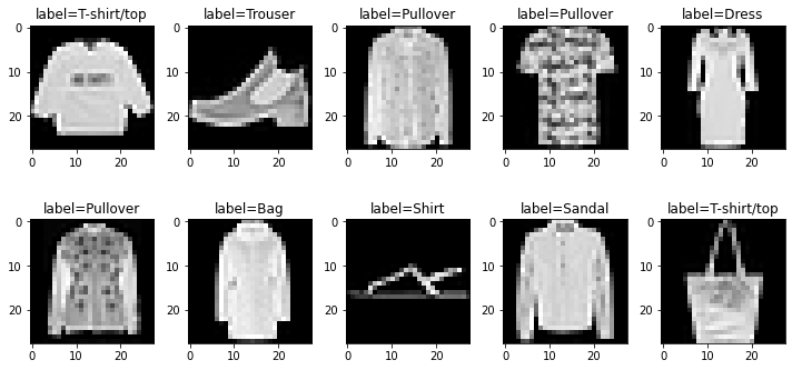

(1) \({\tt xtrain}\)에서 각 라벨에 대한 평균이미지를 계산하고 계산결과를 \({\tt imgmean}\)에 길이가 10인 list로 저장하라. 즉 \({\tt imgmean}\)은 아래와 같은 자료구조를 가지고 있어야 한다.

\({\tt imgmean}=\big[{\tt imgmean[0]},\dots, {\tt imgmean[9]}\big]\)
\({\tt imgmean[0]}, \dots, {\tt imgmean[9]}\) 는 각각 (28,28)의 shape을 가진 numpy array
\({\tt imgmean[0]}, \dots, {\tt imgmean[9]}\) 는 각각 숫자 0,1, …, 9의 평균이미지를 의미

\({\tt imgmean[0]},\dots, {\tt imgmean[9]}\)를 시각화 하라.

(풀이)

imgmean = [xtrain[ytrain==i].mean(axis=0) for i in range(10)] 

fig, ax = plt.subplots(2,5,figsize=(10,5))
ax[0][0].imshow(imgmean[0],cmap='gray'); ax[0][0].set_title('label={}'.format(labels[0]));
ax[0][1].imshow(imgmean[1],cmap='gray'); ax[0][1].set_title('label={}'.format(labels[1]));
ax[0][2].imshow(imgmean[2],cmap='gray'); ax[0][2].set_title('label={}'.format(labels[2]));
ax[0][3].imshow(imgmean[3],cmap='gray'); ax[0][3].set_title('label={}'.format(labels[3]));
ax[0][4].imshow(imgmean[4],cmap='gray'); ax[0][4].set_title('label={}'.format(labels[4]));
ax[1][0].imshow(imgmean[5],cmap='gray'); ax[1][0].set_title('label={}'.format(labels[5]));
ax[1][1].imshow(imgmean[6],cmap='gray'); ax[1][1].set_title('label={}'.format(labels[6]));
ax[1][2].imshow(imgmean[7],cmap='gray'); ax[1][2].set_title('label={}'.format(labels[7]));
ax[1][3].imshow(imgmean[8],cmap='gray'); ax[1][3].set_title('label={}'.format(labels[8]));
ax[1][4].imshow(imgmean[9],cmap='gray'); ax[1][4].set_title('label={}'.format(labels[9]));
fig.tight_layout()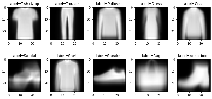

(2) 아래와 같은 numpy array 를 생성하라.

\[{\tt loss}= \begin{bmatrix} {\tt loss[0,0]} & \dots & {\tt loss[0,9]} \\ {\tt loss[1,0]} & \dots & {\tt loss[1,9]} \\ \dots & \dots & \dots \\ {\tt loss[59999,0]}& \dots &{\tt loss[59999,9]} \\ \end{bmatrix}\]

여기에서

\[{\tt loss[i,j]} = \frac{1}{28\times 28} \sum_{p=0}^{27}\sum_{q=0}^{27}\big({\tt xtrain[i,p,q]}-{\tt imgmean[j][p,q]}\big)^2\]

이다. 이제 \({\tt loss}\)에서 “최소값을 가지는 원소의 인덱스를 출력”하는 함수를 행별로 적용해 이미지를 분류하라. 예를들어 모든 \(j=0,1,\dots,9\) 에 대하여 아래를 계산한 결과

\[\frac{1}{28\times 28} \sum_{p=0}^{27}\sum_{q=0}^{27}\big({\tt xtrain[1,p,q]}-{\tt imgmean[j][p,q]}\big)^2\]

\(j=9\)일 경우 그 값이 가장 작다면 \({\tt xtrain[1]}\) 이미지는 9번으로 분류한다. 분류한 결과와 실제 라벨 \({\tt ytrain}\)을 비교하라. 얼마나 많은 결과가 일치하는지 비율을 계산하라.

(풀이)

training_loss = np.array([[np.mean((xtrain[j,:,:]- imgmean[i])**2) for i in range(10)] for j in range(60000)])
ytrain_hat = training_loss.argmin(axis=1)
np.mean(ytrain_hat == ytrain)

0.6850666666666667

(3) \({\tt xtrain}\)에서 학습한 평균이미지 \({\tt imgmean}\)를 바탕으로 \({\tt xtest}\)의 1번라벨에 해당하는 이미지만을 분류하라. 아래의 물음에 답하라.

1번라벨에 해당하는 이미지를 0번라벨로 분류한 경우는 모두 몇건인가? (잘못된 분류)
1번라벨에 해당하는 이미지를 1번라벨로 분류한 경우는 모두 몇건인가? (올바른 분류)
\(\dots\)
1번라벨에 해당하는 이미지를 9번라벨로 분류한 경우는 모두 몇건인가? (잘못된 분류)

hint: 아래와 같은 결과를 주는 dictionary를 만들면 된다.

{0: 28, 1: 895, 2: 11, 3: 36, 4: 8, 5: 12, 6: 10, 7: 0, 8: 0, 9: 0}

1번라벨에 해당하는 이미지를 0번라벨로 분류한 경우는 모두 28건
1번라벨에 해당하는 이미지를 1번라벨로 분류한 경우는 모두 895건
\(\dots\)
1번라벨에 해당하는 이미지를 9번라벨로 분류한 경우는 모두 0건

(풀이)

test_loss = np.array([[np.mean((xtest[j,:,:]- imgmean[i])**2) for i in range(10)] for j in range(10000)])
ytest_hat = test_loss.argmin(axis=1)
{j: ytest_hat[ytest==1].tolist().count(j) for j in range(10)}

{0: 28, 1: 895, 2: 11, 3: 36, 4: 8, 5: 12, 6: 10, 7: 0, 8: 0, 9: 0}

(4) \({\tt xtest}\)의 이미지를 올바르게 분류한 비율을 카테고리별로 정리하라.

(풀이)

{labels[j]:ytest_hat[ytest==j].tolist().count(j)/sum(ytest==j) for j in range(10)}

{'T-shirt/top': 0.7,
 'Trouser': 0.895,
 'Pullover': 0.496,
 'Dress': 0.802,
 'Coat': 0.599,
 'Sandal': 0.757,
 'Shirt': 0.202,
 'Sneaker': 0.794,
 'Bag': 0.761,
 'Ankel boot': 0.851}

3. 파이썬의 설치 (5점)

다음을 읽고 파이썬과 가상환경에 대하여 올바른 진술을 한 사람을 모두 골라라. (모두 맞출 경우만 정답으로 인정함)

민정: 구글코랩은 사용자의 컴퓨터에 설치된 아나콘다를 기반으로 동작하며, 실제적으로는 사용자의 ipython과 크롬과의 통신만을 담당한다. 따라서 구글코랩은 반드시 파이썬만 연결하여 사용가능하지 않으며 실제로 구글코랩에 R을 연결하여 사용하기도 한다.

구환: 아래와 같이 스크립트로 구성된 mysum.py와 같은 파이썬파일을 실행하기 위해서는 반드시 ipython 이나 주피터랩이 설치된 상태이어야 한다.

## mysum.py
total = 0 
for i in range(1,11): 
    total = total + i
print(total)

슬기: 아나콘다를 이용하여 가상환경을 만들 경우 두 가지버전 이상의 python을 동시에 관리할 수 있다.

승민: 아래와 같이 myfuns.py 파일을 구성하였다고 하자.

# myfuns.py
def vec2_add(a,b): 
    return [a[0]+b[0], a[1]+b[1]]

이 경우 아래와 같이 임의의 주피터 노트북에서 myfuns를 임포트하면 vec2_add 함수를 사용할 수 있다.

import myfuns

단, 여기에서 myfuns.py는 현재 실행중인 노트북과 같은 폴더에 있다고 가정한다.

(풀이) 슬기, 승민

민정: 코랩은 사용자의 컴퓨터에 설치된 아나콘다를 기반으로 동작하며 (X)
구환: 반드시 ipython 이나 주피터랩이 설치된 상태이어야 한다. (X)

4. 삼성전자의 주가 추가문제 (30점)

다음은 삼성전자의 주가를 크롤링하는 코드이다.

start_date = "2023-01-01"
end_date = "2023-05-02"
y = yf.download("005930.KS", start=start_date, end=end_date)['Adj Close'].to_numpy()

[*********************100%***********************]  1 of 1 completed

삼성전자의 주가 \({\boldsymbol y}\)를 시각화하면 아래와 같다.

plt.plot(y)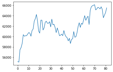

(1) 아래와 같은 \({\bf x}\)를 설정하라.

\[{\bf x}=(x_1,x_2,\dots,x_n)=\big(\frac{1}{n},\frac{2}{n},\dots,1\big)\]

\({\bf x}=(x_1,\dots,x_n)\)을 바탕으로 아래와 같은 매트릭스 \({\bf X}\)를 생성하라. 단, \(n={\tt len}({\boldsymbol y})\).

\[{\bf X}=\begin{bmatrix} 1 & x_1 \\ 1 & x_2\\ \dots & \dots \\ 1 & x_n \end{bmatrix}\]

hint: \({\bf X}\)를 아래와 같이 해석해도 무방하다.

\[{\bf X}=\begin{bmatrix} x_1^0 & x_1^1 \\ x_2^0 & x_2^1\\ \dots & \dots \\ x_n^0 & x_n^1 \end{bmatrix}\]

x = np.arange(1,83)/82 # x = np.arange(0,82)/82 정도의 실수는 정답으로 인정..
X = np.stack([x**k for k in range(2)],axis=1)

(2) (1)에서 계산된 \({\bf X}\)에 대하여 아래를 계산하라.

\[\hat{\bf y}= {\bf X}({\bf X}^T {\bf X})^{-1}{\bf X}^T {\bf y}\]

\((x_i,y_i)\)와 \((x_i,\hat{y}_i)\)을 겹쳐서 시각화하라. 단, \(\hat{\bf y}=(\hat{y}_1,\dots,\hat{y}_n)\).

hint: 계산의 편의를 위하여 \({\bf y}\)와 \(\hat{\bf y}\)은 모두 \(n\times 1\) col-vector가 아닌 길이가 \(n\)인 벡터로 해석해도 무방하다.

(풀이)

yhat= X@np.linalg.inv(X.T@ X)@ X.T @ y
plt.plot(x,y, label=r'$(x_i,y_i)$')
plt.plot(x,yhat,'--',label=r'$(x_i,\hat{y}_i)$')
plt.legend()

<matplotlib.legend.Legend at 0x7f6ebb83c700>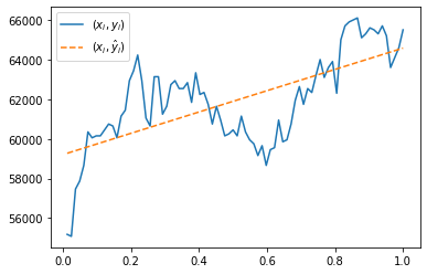

3. 아래와 같이 \({\bf X}\)를 수정하라.

\[{\bf X}=\begin{bmatrix} 1 & x_1 & x_1^2 & x_1^3 & \dots & x_1^{10} \\ 1 & x_2 & x_2^2 & x_2^3 & \dots & x_2^{10} \\ \dots & \dots & \dots & \dots & \dots & \dots \\ 1 & x_n & x_n^2 & x_n^3 & \dots & x_n^{10} \end{bmatrix}\]

수정된 \({\bf X}\)에 대하여 아래의 수식으로 \(\hat{\bf y}\)을 구하라.

\[\hat{\bf y}= {\bf X}({\bf X}^T {\bf X})^{-1}{\bf X}^T {\bf y}\]

\((x_i,y_i)\)와 \((x_i,\hat{y}_i)\)을 겹쳐서 시각화하라. 단, \(\hat{\bf y}=(\hat{y}_1,\dots,\hat{y}_n)\).

(풀이)

X = np.stack([x**k for k in range(11)],axis=1)
plt.plot(x,y, label=r'$(x_i,y_i)$')
plt.plot(x, X@np.linalg.inv(X.T@ X)@ X.T @ y,'--',label=r'$(x_i,\hat{y}_i)$')
plt.legend()

<matplotlib.legend.Legend at 0x7f6ebb7cd370>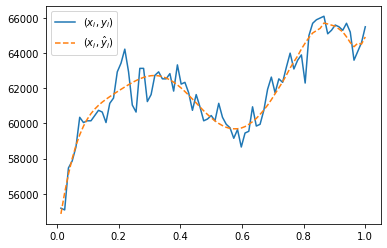

5. fashin MNIST data 추가문제 (30점)

이 문제는 2번문항의 추가문항입니다.

# read data 
df_train=pd.read_csv('https://media.githubusercontent.com/media/guebin/PP2023/main/posts/fashion-mnist_train.csv')
df_test=pd.read_csv('https://media.githubusercontent.com/media/guebin/PP2023/main/posts/fashion-mnist_test.csv')

# rshp 함수정의 
def rshp(row):
    return row.reshape(28,28)

# cleaning data 
xtrain = np.apply_along_axis(rshp,axis=1,arr=np.array(df_train.iloc[:,1:]))
xtest  = np.apply_along_axis(rshp,axis=1,arr=np.array(df_test.iloc[:,1:]))
ytrain = np.array(df_train.label)
ytest  = np.array(df_test.label)

\({\tt imgmean}=\big[{\tt imgmean[0]},\dots, {\tt imgmean[9]}\big]\)
\({\tt imgmean[0]}, \dots, {\tt imgmean[9]}\) 는 각각 (28,28)의 shape을 가진 numpy array
\({\tt imgmean[0]}, \dots, {\tt imgmean[9]}\) 는 각각 숫자 0,1, …, 9의 평균이미지를 의미

모든 \(i=0,\dots,9\)에 대하여 아래를 계산하고

\[{\tt dist}[i] = \frac{1}{28\times 28} \sum_{p=0}^{27}\sum_{q=0}^{27}\big({\tt imgmean}[2][p,q]-{\tt imgmean}[i][p,q]\big)^2\]

\({\tt dist}[i]\)의 값이 가장 작은 \(i\)를 찾아라. 단 \({\tt dist}[i]=0\) 인 경우는 제외한다. (즉 2번 라벨과 평균이미지가 가장 비슷한 카테고리를 찾아라)

hint: 4번라벨이 2번라벨과 가장 비슷하다.

(풀이1)

imgmean = [xtrain[ytrain==i].mean(axis=0) for i in range(10)] 
[np.mean((imgmean[i] - imgmean[2])**2) for i in range(10)]

[2597.2085496295,
 5878.065097639916,
 0.0,
 4213.533631714888,
 498.11027318129953,
 7492.365150424071,
 565.4023419996103,
 8216.785686526042,
 2762.121757294324,
 6135.9385566330075]

(풀이2)

imgmean = [xtrain[ytrain==i].mean(axis=0) for i in range(10)] 
np.mean((imgmean - imgmean[2])**2,axis=(1,2))

array([2597.20854963, 5878.06509764,    0.        , 4213.53363171,
        498.11027318, 7492.36515042,  565.402342  , 8216.78568653,
       2762.12175729, 6135.93855663])

(2) (1)의 과정을 반복하여 아래의 평균이미지를 비슷한 카테고리로 묶는 작업을 하였다고 하자.

# 평균이미지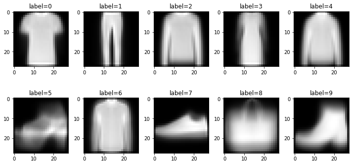

작업결과 아래와 같이 비슷한 카테고리를 생각하였다고 하자.

mapping_rule = {0:[0,2,3,4,6], 1:[1], 2:[5,7,9], 3:[8]}
mapping_rule

{0: [0, 2, 3, 4, 6], 1: [1], 2: [5, 7, 9], 3: [8]}

즉 기존의 0,2,3,4,6번에 해당하는 이미지는 모두 비슷하다고 판단하였다. 위에 제시된 mapping_rule에 의거하여 아래와 같이 라벨의 수정하는 변환을 수행하라.

Before	After
0	0
1	1
2	0
3	0
4	0
5	2
6	0
7	2
8	3
9	2

수정된 라벨에 대하여 평균이미지를 다시 계산하여 imgmean2에 저장하고 아래의 코드를 이용하여 시각화하라.

fig, ax = plt.subplots(1,4,figsize=(10,5))
for i in range(4):
    ax[i].imshow(imgmean2[i],cmap='gray')

(풀이1)

ytrain2 = np.array([m for y in ytrain for m in mapping_rule if y in mapping_rule[m]])

imgmean2 = [xtrain[ytrain2==i].mean(axis=0) for i in range(4)]

fig, ax = plt.subplots(1,4,figsize=(10,5))
for i in range(4):
    ax[i].imshow(imgmean2[i],cmap='gray')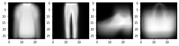

(풀이2)

inv = {v:k for k in mapping_rule for v in mapping_rule[k]}
inv

{0: 0, 2: 0, 3: 0, 4: 0, 6: 0, 1: 1, 5: 2, 7: 2, 9: 2, 8: 3}

ytrain2 = np.array([inv[y] for y in ytrain])

imgmean2 = [xtrain[ytrain2==i].mean(axis=0) for i in range(4)]

fig, ax = plt.subplots(1,4,figsize=(10,5))
for i in range(4):
    ax[i].imshow(imgmean2[i],cmap='gray')

(3) 수정된 라벨에 대하여 xtrain의 이미지를 분류하고 분류결과를 카테고리별로 제시하라.

(풀이1)

training_loss2 = np.array([[np.mean((xtrain[j,:,:]- imgmean2[i])**2) for i in range(4)] for j in range(60000)])
ytrain2_hat = training_loss2.argmin(axis=1)
{i:ytrain2_hat[ytrain2==i].tolist().count(i)/sum(ytrain2==i) for i in range(4)}

{0: 0.7493333333333333,
 1: 0.9443333333333334,
 2: 0.9379444444444445,
 3: 0.7983333333333333}

(풀이2)

training_loss2 = np.array([[np.mean((xtrain[j,:,:]- imgmean2[i])**2) for i in range(4)] for j in range(60000)])
ytrain2_hat = training_loss2.argmin(axis=1)

[np.mean(ytrain2_hat[ytrain2==i]==i) for i in range(4)]

[0.7493333333333333,
 0.9443333333333334,
 0.9379444444444445,
 0.7983333333333333]

6. 동물명: 최하니 (20점)

아래는 동물명 “최하니”의 이미지이다.

url = 'https://raw.githubusercontent.com/guebin/SC2022/main/hani.jpeg'
hani = np.einsum('ijk->jik',np.array(PIL.Image.open(io.BytesIO(requests.get(url).content))),dtype=np.int64)/255

plt.imshow(hani)

<matplotlib.image.AxesImage at 0x7f6efc778130>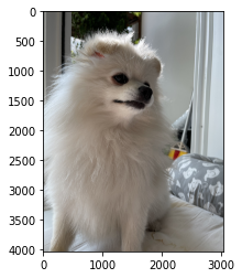

아래는 하니를 적당히 분리하여 아래와 같이 hani_left와 hini_right를 만들고 시각화한 것이다.

hani_left = hani[:,:1512,:].copy()
hani_right = hani[:,1512:,:].copy()

fig, ax = plt.subplots(1,2)
ax[0].imshow(hani_left)
ax[1].imshow(hani_right)

<matplotlib.image.AxesImage at 0x7f6ebb92b280>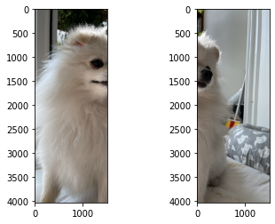

(1) hani_right[:,:,2]의 모든 원소에 아래와 같은 변환을 수행하라.

\(f(x)=\begin{cases} x & 1.15x >1.0 \\ 1.15x & 1.15x \leq 1.0 \end{cases}\)

(풀이1)

_a = hani_right[:,:,2] * (hani_right[:,:,2]*1.15 > 1.0)
_b = hani_right[:,:,2]*1.15 * (hani_right[:,:,2]*1.15 < 1.0)
hani_right[:,:,2] = _a + _b

(풀이2)

def f(x): 
    if 1.15*x > 1.0:
        return x 
    else: 
        return 1.15*x

for i in range(4023):
    for j in range(1512):
        hani_right[i,j,2] = f(hani_right[i,j,2])

(2) hani_left와 (1)에서 변환된 hani_right를 np.concatenate을 이용하여 합치고 결과를 시각화하라.

(풀이)

plt.imshow(np.concatenate([hani_left,hani_right],axis=1))

<matplotlib.image.AxesImage at 0x7f6ebae56c10>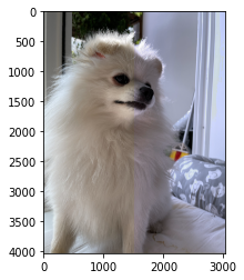

7. Naive Bayes classifier (120점)

ref: https://towardsdatascience.com/the-naive-bayes-classifier-how-it-works-e229e7970b84

아래의 데이터프레임은 날씨, 도로 상태, 교통 상황, 엔진 문제 및 사고 여부와 같은 여러 가지 변수를 포함하는 10개의 행과 5개의 열로 구성되어있다.

df = pd.DataFrame({
    'WeatherCondition': ['rain', 'snow', 'clear', 'clear', 'snow', 'rain', 'rain', 'snow', 'clear', 'clear'],
    'RoadCondition': ['bad','average','bad','good','good','average','good','bad','good','bad'],
    'TrafficCondition': ['high','normal','light','light','normal','light','normal','high','high','high'],
    'EngineProblem': ['no','yes','no','yes','no','no','no','no','yes','yes'],
    'Accident': ['yes','yes','no','yes','no','no','no','yes','no','yes']
})

df

	WeatherCondition	RoadCondition	TrafficCondition	EngineProblem	Accident
0	rain	bad	high	no	yes
1	snow	average	normal	yes	yes
2	clear	bad	light	no	no
3	clear	good	light	yes	yes
4	snow	good	normal	no	no
5	rain	average	light	no	no
6	rain	good	normal	no	no
7	snow	bad	high	no	yes
8	clear	good	high	yes	no
9	clear	bad	high	yes	yes

각 열에 대한 설명은 아래와 같다.

‘WeatherCondition’: 각 행에서 기록된 날씨 조건을 설명하며, ’rain’은 비, ’snow’는 눈, ’clear’는 맑은 날씨를 나타낸다.
‘RoadCondition’:각 행에서 기록된 도로 상태를 설명하며, ’bad’는 안 좋은, ’average’는 보통, ’good’은 좋은 도로 상태를 나타낸다.
‘TrafficCondition’:각 행에서 기록된 교통 상황을 설명하며, ’light’는 움직이기 쉬운, ’normal’은 평균, ’high’는 교통이 많은 상황을 나타낸다.
‘EngineProblem’: 각 행에서 기록된 엔진 문제 여부를 설명하며, ’yes’는 문제가 있음을 나타내고, ’no’는 문제가 없음을 나타낸다.
‘Accident’: 각 행에서 기록된 사고 여부를 설명하며, ’yes’는 사고가 있음을 나타내고, ’no’는 사고가 없음을 나타낸다.

우리는 ‘WeatherCondition’, ‘RoadCondition’, ‘TrafficCondition’, ‘EngineProblem’ 를 이용하여 ‘Accident’ 행의 값이 yes일지 no일지를 판단하는 일에 관심이 있다고 하자. 아래의 (1)-(4) 이러한 분류를 수행하는 방법을 구체화 한 것이다. (1)-(4)의 물음에 답하라.

(1) 주어진 자료에서 \(P({\tt Accident == no})\)를 계산하여라.

hint: Accident=='no'인 데이터수 / 전체데이터수를 계산하면 되며 답은 0.5이다.

(풀이)

len(df.query('Accident=="no"')) / 10

0.5

(2) 아래와 같은 조건부 확률은

\[P({\tt WeatherCondition == rain} ~|~ {\tt Accident==no})\]

아래와 같이 계산한다고 하자.

# 방법1
len(df.query('WeatherCondition == "rain" and Accident == "no"'))/len(df.query('Accident=="no"'))

0.4

# 방법2
((df['WeatherCondition'] == 'rain') & (df['Accident']== 'no')).sum() / (df['Accident']== 'no').sum()

0.4

이와 유사한 방식으로 아래를 계산하라.

\(P({\tt WeatherCondition == rain} ~|~ {\tt Accident==no})\)
\(P({\tt WeatherCondition == snow} ~|~ {\tt Accident==no})\)
\(\dots\)
\(P({\tt EngineProblem == no} ~|~ {\tt Accident==yes})\)
\(P({\tt EngineProblem == yes} ~|~ {\tt Accident==yes})\)

(풀이1)

*cond, _ = df.columns
{'P({}={}|Accident={})'.format(i,j,k): ((df[i]==j)&(df['Accident']==k)).sum()/(df['Accident']==k).sum() for i in cond for j in set(df[i]) for k in ['no','yes']}

{'P(WeatherCondition=clear|Accident=no)': 0.4,
 'P(WeatherCondition=clear|Accident=yes)': 0.4,
 'P(WeatherCondition=rain|Accident=no)': 0.4,
 'P(WeatherCondition=rain|Accident=yes)': 0.2,
 'P(WeatherCondition=snow|Accident=no)': 0.2,
 'P(WeatherCondition=snow|Accident=yes)': 0.4,
 'P(RoadCondition=average|Accident=no)': 0.2,
 'P(RoadCondition=average|Accident=yes)': 0.2,
 'P(RoadCondition=bad|Accident=no)': 0.2,
 'P(RoadCondition=bad|Accident=yes)': 0.6,
 'P(RoadCondition=good|Accident=no)': 0.6,
 'P(RoadCondition=good|Accident=yes)': 0.2,
 'P(TrafficCondition=normal|Accident=no)': 0.4,
 'P(TrafficCondition=normal|Accident=yes)': 0.2,
 'P(TrafficCondition=light|Accident=no)': 0.4,
 'P(TrafficCondition=light|Accident=yes)': 0.2,
 'P(TrafficCondition=high|Accident=no)': 0.2,
 'P(TrafficCondition=high|Accident=yes)': 0.6,
 'P(EngineProblem=yes|Accident=no)': 0.2,
 'P(EngineProblem=yes|Accident=yes)': 0.6,
 'P(EngineProblem=no|Accident=no)': 0.8,
 'P(EngineProblem=no|Accident=yes)': 0.4}

(풀이2)

dct = {(j,k):((df[i]==j)&(df['Accident']==k)).sum()/(df['Accident']==k).sum() for i in cond for j in set(df[i]) for k in ['no','yes']}
dct

{('clear', 'no'): 0.4,
 ('clear', 'yes'): 0.4,
 ('rain', 'no'): 0.4,
 ('rain', 'yes'): 0.2,
 ('snow', 'no'): 0.2,
 ('snow', 'yes'): 0.4,
 ('average', 'no'): 0.2,
 ('average', 'yes'): 0.2,
 ('bad', 'no'): 0.2,
 ('bad', 'yes'): 0.6,
 ('good', 'no'): 0.6,
 ('good', 'yes'): 0.2,
 ('normal', 'no'): 0.4,
 ('normal', 'yes'): 0.2,
 ('light', 'no'): 0.4,
 ('light', 'yes'): 0.2,
 ('high', 'no'): 0.2,
 ('high', 'yes'): 0.6,
 ('yes', 'no'): 0.2,
 ('yes', 'yes'): 0.6,
 ('no', 'no'): 0.8,
 ('no', 'yes'): 0.4}

(3) 아래와 같은 새로운 상황이 발생하였다고 가정하자.

\({\tt WeatherCondition==rain}\)
\({\tt RoadCondition==good}\)
\({\tt TraffictCondition==normal}\)
\({\tt EngineProblem==no}\)

아래를 각각 계산하라.

\(\begin{align} A&=P({\tt Accident == yes})\\ &\times P({\tt WeatherCondition==rain~ |~ Accident == yes}) \\ &\times P({\tt RoadCondition==good~|~ Accident == yes}) \\ &\times P({\tt TrafficCondition==normal~ |~ Accident == yes}) \\ &\times P({\tt EngineProblem=no~ |~ Accident == yes}) \end{align}\)

\(\begin{align} B&=P({\tt Accident ==no})\\ &\times P({\tt WeatherCondition==rain~ |~ Accident == no}) \\ &\times P({\tt RoadCondition==good~|~ Accident == no}) \\ &\times P({\tt TrafficCondition==normal~ |~ Accident == no}) \\ &\times P({\tt EngineProblem=no~ |~ Accident == no}) \end{align}\)

여기에서 \(\frac{A}{A+B}\)와 \(\frac{B}{A+B}\)를 각각 주어진 상황에 대하여 사고가 날 확률, 사고가 나지 않을 확률을 의미한다고 하자. 주어진 상황에서 사고가 날 확률은 얼마인가?

hint: 답은 1/25

(풀이)

dct = {(j,k):((df[i]==j)&(df['Accident']==k)).sum()/(df['Accident']==k).sum() for i in cond for j in set(df[i]) for k in ['no','yes']}
dct

{('clear', 'no'): 0.4,
 ('clear', 'yes'): 0.4,
 ('rain', 'no'): 0.4,
 ('rain', 'yes'): 0.2,
 ('snow', 'no'): 0.2,
 ('snow', 'yes'): 0.4,
 ('average', 'no'): 0.2,
 ('average', 'yes'): 0.2,
 ('bad', 'no'): 0.2,
 ('bad', 'yes'): 0.6,
 ('good', 'no'): 0.6,
 ('good', 'yes'): 0.2,
 ('normal', 'no'): 0.4,
 ('normal', 'yes'): 0.2,
 ('light', 'no'): 0.4,
 ('light', 'yes'): 0.2,
 ('high', 'no'): 0.2,
 ('high', 'yes'): 0.6,
 ('yes', 'no'): 0.2,
 ('yes', 'yes'): 0.6,
 ('no', 'no'): 0.8,
 ('no', 'yes'): 0.4}

dct의 키는 (WeatherCondition~EngineProblem의 라벨, Accident의 라벨)로 이루어짐

A = dct['rain','yes']*dct['good','yes']*dct['normal','yes']*dct['no','yes']
B = dct['rain','no']*dct['good','no']*dct['normal','no']*dct['no','no']

A/(A+B) # 실제정답은 0.04, 0.000000000000000015는 에러

0.040000000000000015

(4) 모든 상황에 대하여 사고가 날 확률을 구하여라.

(풀이1)

W = set(df.WeatherCondition)
R = set(df.RoadCondition)
T = set(df.TrafficCondition)
E = set(df.EngineProblem)

df2 = pd.DataFrame([[w,r,t,e,dct[w,'yes']*dct[r,'yes']*dct[t,'yes']*dct[e,'yes'],dct[w,'no']*dct[r,'no']*dct[t,'no']*dct[e,'no']] for w in W for r in R for t in T for e in E])
df2.columns = pd.Index(['WeatherCondition','RoadCondition','TrafficCondition','EngineProblem','A','B'])
df2.eval('Prob = A/(A+B)')

	WeatherCondition	RoadCondition	TrafficCondition	EngineProblem	A	B	Prob
0	clear	average	normal	yes	0.0096	0.0064	0.600000
1	clear	average	normal	no	0.0064	0.0256	0.200000
2	clear	average	light	yes	0.0096	0.0064	0.600000
3	clear	average	light	no	0.0064	0.0256	0.200000
4	clear	average	high	yes	0.0288	0.0032	0.900000
5	clear	average	high	no	0.0192	0.0128	0.600000
6	clear	bad	normal	yes	0.0288	0.0064	0.818182
7	clear	bad	normal	no	0.0192	0.0256	0.428571
8	clear	bad	light	yes	0.0288	0.0064	0.818182
9	clear	bad	light	no	0.0192	0.0256	0.428571
10	clear	bad	high	yes	0.0864	0.0032	0.964286
11	clear	bad	high	no	0.0576	0.0128	0.818182
12	clear	good	normal	yes	0.0096	0.0192	0.333333
13	clear	good	normal	no	0.0064	0.0768	0.076923
14	clear	good	light	yes	0.0096	0.0192	0.333333
15	clear	good	light	no	0.0064	0.0768	0.076923
16	clear	good	high	yes	0.0288	0.0096	0.750000
17	clear	good	high	no	0.0192	0.0384	0.333333
18	rain	average	normal	yes	0.0048	0.0064	0.428571
19	rain	average	normal	no	0.0032	0.0256	0.111111
20	rain	average	light	yes	0.0048	0.0064	0.428571
21	rain	average	light	no	0.0032	0.0256	0.111111
22	rain	average	high	yes	0.0144	0.0032	0.818182
23	rain	average	high	no	0.0096	0.0128	0.428571
24	rain	bad	normal	yes	0.0144	0.0064	0.692308
25	rain	bad	normal	no	0.0096	0.0256	0.272727
26	rain	bad	light	yes	0.0144	0.0064	0.692308
27	rain	bad	light	no	0.0096	0.0256	0.272727
28	rain	bad	high	yes	0.0432	0.0032	0.931034
29	rain	bad	high	no	0.0288	0.0128	0.692308
30	rain	good	normal	yes	0.0048	0.0192	0.200000
31	rain	good	normal	no	0.0032	0.0768	0.040000
32	rain	good	light	yes	0.0048	0.0192	0.200000
33	rain	good	light	no	0.0032	0.0768	0.040000
34	rain	good	high	yes	0.0144	0.0096	0.600000
35	rain	good	high	no	0.0096	0.0384	0.200000
36	snow	average	normal	yes	0.0096	0.0032	0.750000
37	snow	average	normal	no	0.0064	0.0128	0.333333
38	snow	average	light	yes	0.0096	0.0032	0.750000
39	snow	average	light	no	0.0064	0.0128	0.333333
40	snow	average	high	yes	0.0288	0.0016	0.947368
41	snow	average	high	no	0.0192	0.0064	0.750000
42	snow	bad	normal	yes	0.0288	0.0032	0.900000
43	snow	bad	normal	no	0.0192	0.0128	0.600000
44	snow	bad	light	yes	0.0288	0.0032	0.900000
45	snow	bad	light	no	0.0192	0.0128	0.600000
46	snow	bad	high	yes	0.0864	0.0016	0.981818
47	snow	bad	high	no	0.0576	0.0064	0.900000
48	snow	good	normal	yes	0.0096	0.0096	0.500000
49	snow	good	normal	no	0.0064	0.0384	0.142857
50	snow	good	light	yes	0.0096	0.0096	0.500000
51	snow	good	light	no	0.0064	0.0384	0.142857
52	snow	good	high	yes	0.0288	0.0048	0.857143
53	snow	good	high	no	0.0192	0.0192	0.500000

(풀이2) – 좀 더 일반적인 풀이

import itertools
lst = []
for cond_details in itertools.product(*[set(df[col_name]) for col_name in cond]):
    A=1;
    B=1;
    for c in cond_details:
        A = A* dct[c,'yes']
        B = B*dct[c,'no']
    lst.append([*cond_details,A,B,A/(A+B)])

df2 = pd.DataFrame(lst)
df2.columns = pd.Index(['WeatherCondition','RoadCondition','TrafficCondition','EngineProblem','A','B','Prob'])
df2

	WeatherCondition	RoadCondition	TrafficCondition	EngineProblem	A	B	Prob
0	clear	average	normal	yes	0.0096	0.0064	0.600000
1	clear	average	normal	no	0.0064	0.0256	0.200000
2	clear	average	light	yes	0.0096	0.0064	0.600000
3	clear	average	light	no	0.0064	0.0256	0.200000
4	clear	average	high	yes	0.0288	0.0032	0.900000
5	clear	average	high	no	0.0192	0.0128	0.600000
6	clear	bad	normal	yes	0.0288	0.0064	0.818182
7	clear	bad	normal	no	0.0192	0.0256	0.428571
8	clear	bad	light	yes	0.0288	0.0064	0.818182
9	clear	bad	light	no	0.0192	0.0256	0.428571
10	clear	bad	high	yes	0.0864	0.0032	0.964286
11	clear	bad	high	no	0.0576	0.0128	0.818182
12	clear	good	normal	yes	0.0096	0.0192	0.333333
13	clear	good	normal	no	0.0064	0.0768	0.076923
14	clear	good	light	yes	0.0096	0.0192	0.333333
15	clear	good	light	no	0.0064	0.0768	0.076923
16	clear	good	high	yes	0.0288	0.0096	0.750000
17	clear	good	high	no	0.0192	0.0384	0.333333
18	rain	average	normal	yes	0.0048	0.0064	0.428571
19	rain	average	normal	no	0.0032	0.0256	0.111111
20	rain	average	light	yes	0.0048	0.0064	0.428571
21	rain	average	light	no	0.0032	0.0256	0.111111
22	rain	average	high	yes	0.0144	0.0032	0.818182
23	rain	average	high	no	0.0096	0.0128	0.428571
24	rain	bad	normal	yes	0.0144	0.0064	0.692308
25	rain	bad	normal	no	0.0096	0.0256	0.272727
26	rain	bad	light	yes	0.0144	0.0064	0.692308
27	rain	bad	light	no	0.0096	0.0256	0.272727
28	rain	bad	high	yes	0.0432	0.0032	0.931034
29	rain	bad	high	no	0.0288	0.0128	0.692308
30	rain	good	normal	yes	0.0048	0.0192	0.200000
31	rain	good	normal	no	0.0032	0.0768	0.040000
32	rain	good	light	yes	0.0048	0.0192	0.200000
33	rain	good	light	no	0.0032	0.0768	0.040000
34	rain	good	high	yes	0.0144	0.0096	0.600000
35	rain	good	high	no	0.0096	0.0384	0.200000
36	snow	average	normal	yes	0.0096	0.0032	0.750000
37	snow	average	normal	no	0.0064	0.0128	0.333333
38	snow	average	light	yes	0.0096	0.0032	0.750000
39	snow	average	light	no	0.0064	0.0128	0.333333
40	snow	average	high	yes	0.0288	0.0016	0.947368
41	snow	average	high	no	0.0192	0.0064	0.750000
42	snow	bad	normal	yes	0.0288	0.0032	0.900000
43	snow	bad	normal	no	0.0192	0.0128	0.600000
44	snow	bad	light	yes	0.0288	0.0032	0.900000
45	snow	bad	light	no	0.0192	0.0128	0.600000
46	snow	bad	high	yes	0.0864	0.0016	0.981818
47	snow	bad	high	no	0.0576	0.0064	0.900000
48	snow	good	normal	yes	0.0096	0.0096	0.500000
49	snow	good	normal	no	0.0064	0.0384	0.142857
50	snow	good	light	yes	0.0096	0.0096	0.500000
51	snow	good	light	no	0.0064	0.0384	0.142857
52	snow	good	high	yes	0.0288	0.0048	0.857143
53	snow	good	high	no	0.0192	0.0192	0.500000