import numpy as np
import pandas as pd
import matplotlib.pyplot as plt
import urllib.request09wk-1: Numpy와 Pandas의 활용
![]()
강의영상
youtube: https://youtube.com/playlist?list=PLQqh36zP38-w-stglh0uVkQxHpCT9lH9C
imports
회귀분석
1--7.
1. \(x_i\)가 아래와 같이 주어졌다고 가정하자.
x =  np.array([0.00983, 0.01098, 0.02951, 0.0384 , 0.03973, 0.04178, 0.0533 ,
               0.058  , 0.09454, 0.1103 , 0.1328 , 0.1412 , 0.1497 , 0.1664 ,
               0.1906 , 0.1923 , 0.198  , 0.2141 , 0.2393 , 0.2433 , 0.3157 ,
               0.3228 , 0.3418 , 0.3552 , 0.3918 , 0.3962 , 0.4    , 0.4482 ,
               0.496  , 0.507  , 0.53   , 0.5654 , 0.582  , 0.5854 , 0.5854 ,
               0.6606 , 0.7007 , 0.723  , 0.7305 , 0.7383 , 0.7656 , 0.7725 ,
               0.831  , 0.8896 , 0.9053 , 0.914  , 0.949  , 0.952  , 0.9727 ,
               0.982  ])
아래의 수식에 따라 \(y_i\)를 생성하라.
- \(y_i = 2+3x_i +\epsilon_i,\quad \epsilon_i \overset{iid}{\sim} N(0,1)\)
\((x_i,y_i)\)를 산점도를 이용하여 시각화하라.
(풀이)
y = 2+3*x + np.random.randn(50) plt.plot(x,y,'o',label=r'$(x_i,y_i)$')
plt.legend()<matplotlib.legend.Legend at 0x7f457a486790>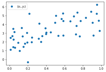
2. 1과 같은 자료를 잘 표현할 수 있는 적절한 추세선 \((x_i, \hat{y}_i)\)를 그리기 위하여 아래의 수식을 고려하자.
- \(\hat{y}_i = ax_i+b\)
a,b를 각각 아래의 표에 의하여 선택하였을 경우 추세선을 문제하단에 명시된 요구사항에 맞추어 시각화하라.
| \(a\) | \(b\) | |
|---|---|---|
| (a) | \(1\) | \(0\) |
| (b) | \(2.5\) | \(2\) |
| (c) | \(3\) | \(2\) |
요구사항
- \((x_i,y_i)\)를 산점도로 그리고 각 (a),(b),(c)에 대한 \((x_i,\hat{y}_i)\)를 lineplot으로 겹쳐그릴 것
- 범례를 포함할 것
plt.plot(x,y,'o',label=r'$(x_i,y_i)$')
plt.plot(x,1*x+0,'--',label=r'(a) $(x_i,\hat{y}_i)$')
plt.plot(x,2.5*x+2,'--',label=r'(b) $(x_i,\hat{y}_i)$')
plt.plot(x,3*x+2,'--',label=r'(c) $(x_i,\hat{y}_i)$')
plt.legend()
<matplotlib.legend.Legend at 0x7f4579b17520>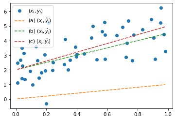
3. 아래를 각각 계산하라.
(a) \(\frac{1}{n}\sum_{i=1}^{n}(y_i-x_i)^2\)
(b) \(\frac{1}{n}\sum_{i=1}^{n}(y_i-2-2.5x_i)^2\)
(c) \(\frac{1}{n}\sum_{i=1}^{n}(y_i-2-3x_i)^2\)
가장 작은 값을 가지는 것은 무엇인가?
(풀이)
np.mean((y-(1*x+0))**2), np.mean((y-(2.5*x+2))**2), np.mean((y-(3*x+2))**2)(9.310962556625569, 1.1267147296257563, 1.0907585903281032)가장 작은 값을 가지는 것은 (c)이다.
4. 3의 결과를 근거로 (a)-(c)중 가장 적절한 추세선을 판단하고 적절한 순서대로 나열하라.
(풀이)
3-(a),(b),(c)는 각각
- \(\hat{y}_i=x_i\)
- \(\hat{y}_i=2+2.5x_i\)
- \(\hat{y}_i=2+3x_i\)
일 경우
\[{\tt mse}({\boldsymbol y}, \hat{\boldsymbol y}) = \frac{1}{n}\sum_{i=1}^{n}(y_i -\hat{y}_i)^2\]
를 계산한 것이라 해석할 수 있다. 그런데 \({\tt mse}({\boldsymbol y}, \hat{\boldsymbol y})\)의 값은
- \(y_1 \approx \hat{y}_1\)
- \(y_2 \approx \hat{y}_2\)
- \(\dots\)
- \(y_n \approx \hat{y}_n\)
일수록 작은 값을 가진다. 그리고 위의 조건은 더 적절하게 추세선을 그렸을때 만족된다. 요약하면
- 적절한 추세선을 그림 \(\Rightarrow\) \(y_i \approx \hat{y}_i\) \(\Rightarrow\) \({\tt mse}({\boldsymbol y}, \hat{\boldsymbol y})\) 값이 작아짐
와 같은 관계가 있음을 파악할 수 있다. 따라서 \({\tt mse}({\boldsymbol y}, \hat{\boldsymbol y})\)의 값이 작을수록 적절한 추세선이라 생각할 수 있다.
5. 아래와 같은 수식을 이용하여 \(\hat{\beta}_0, \hat{\beta}_1\) 을 계산하라.
\[\begin{bmatrix} \hat{\beta}_0 \\ \hat{\beta}_1 \end{bmatrix} = ({\bf X}^T {\bf X})^{-1}{\bf X}^T {\boldsymbol y}, \quad {\bf X}=\begin{bmatrix} 1 & x_1 \\ 1 & x_2 \\ \dots \\ 1 & x_n \end{bmatrix}\]
(풀이)
X = np.stack([[1]*50 ,x],axis=1)
np.linalg.inv(X.T @ X)@X.T@y
array([1.97914281, 2.90834079])\(\hat{\beta}_0=1.97914281\) 이고 \(\hat{\beta}_1= 2.90834079\) 이다.
6. 5에서 계산된 \(\hat{\beta}_0, \hat{\beta}_1\)을 각각 \(b=\hat{\beta}_0, a=\hat{\beta}_1\)으로 생각하고 적절한 추세선 \((x_i, \hat{y}_i)\)를 그려라. (단, \(\hat{y}_i=ax_i+b\) 이다)
(풀이)
b, a = np.linalg.inv(X.T @ X)@X.T@y
yhat = a*x +b plt.plot(x,y,'o',label=r'$(x_i,y_i)$')
plt.plot(x,yhat,'--',label=r'$(x_i,\hat{y}_i)$')
plt.legend()<matplotlib.legend.Legend at 0x7f4577dd45e0>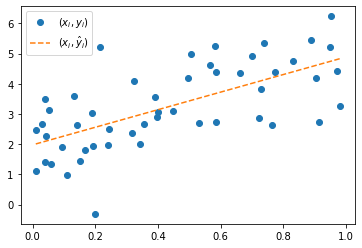
7. 4의 기준에 따르면, \((a,b)=(3,2)\) 일때 만들어지는 추세선과 \((a,b)=(\hat{\beta}_1,\hat{\beta}_0)\) 일때 만들어지는 추세선은 어떤 것이 더 적절한가?
(풀이)
np.mean((y-(3*x+2))**2), np.mean((y-yhat)**2)(1.0907585903281032, 1.0862796480117118)MNIST data
아래는 0~9가지의 숫자이미지가 저장된 이미지데이터를 불러오는 코드이다.
# URL 설정
url = 'https://github.com/guebin/PP2023/raw/main/posts/02_PY4DS/mnist.npz'

# URL에서 파일 다운로드
urllib.request.urlretrieve(url, './mnist.npz')

# 데이터 로드
data = np.load('./mnist.npz')
xtrain, ytrain, xtest, ytest = data['x_train'], data['y_train'], data['x_test'], data['y_test']
아래는 데이터에 대한 설명이다.
- 전체의 이미지의 수는 70000개이며, 60000개의 이미지 \({\tt xtrain}\)에 10000개의 이미지는 \({\tt xtest}\)에 저장되어 있다.
- 이미지에 대한 라벨은 각각 \({\tt ytrain}\)과 \(\tt ytest\)에 저장되어 있다. 따라서 \(\tt ytrain\)에는 60000개의 이미지에 해당하는 라벨이, \(\tt ytest\)에는 10000개의 이미지에 해당하는 라벨이 기록되어 있다.
- 보통 분석에서는 60000개의 이미지를 가지고 라벨을 맞추는 “훈련”을 하고 (\({\tt xtrain}\)을 이용하여 \({\tt ytrain}\)을 맞추는 방법을 학습하고), 그러한 훈련이 잘 되었는지 10000개의 이미지를 이용하여 “테스트”한다.
- 위와 같은 의미로 \(({\tt xtrain}, {\tt ytrain})\) 을 training data set, \(({\tt xtest},{\tt ytest})\) 를 test data set 이라고 부른다. (ref: 위키참고)
아래는 이미지자료와 시각화에 대한 설명이다.
- 각 이미지는 (28,28) 픽셀의 흑백이미지이다. 따라서 각 이미지는 (28,28,3) 이 아니라 (28,28) 의 shape을 가진 텐서로 구성되어있다.
- 흑백이미지를 시각화 하기 위해서는
plt.imshow(img, cmap='gray')를 이용한다. 여기에서 \({\tt img}\)은 임의의 2차원 텐서이며 이 예제의 경우 (28,28)의 shape을 가진다.
아래는 \({\tt xtrain}\)의 두번째 이미지, 즉 \({\tt xtrain[1,:,:]}\)를 확인하는 코드의 예시이다.
# plt.imshow(xtrain[1,:,:],cmap='gray')
plt.imshow(xtrain[1],cmap='gray') ## 같은코드임
<matplotlib.image.AxesImage at 0x7f457418ca30>
이 이미지에 대한 label은 \({\tt ytrain[1]}\)의 값으로 확인가능하다.
ytrain[1]0이미지와 라벨을 한번에 표현하는 코드는 아래와 같이 작성가능하다.
plt.imshow(xtrain[1],cmap='gray')
plt.title('label={}'.format(ytrain[1]));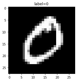
아래는 10개의 이미지를 라벨과 함께 출력하는 코드의 예시이다.
fig, ax = plt.subplots(2,5,figsize=(10,5))

ax[0][0].imshow(xtrain[0],cmap='gray'); ax[0][0].set_title('label={}'.format(ytrain[0]));
ax[0][1].imshow(xtrain[1],cmap='gray'); ax[0][1].set_title('label={}'.format(ytrain[1]));
ax[0][2].imshow(xtrain[2],cmap='gray'); ax[0][2].set_title('label={}'.format(ytrain[2]));
ax[0][3].imshow(xtrain[3],cmap='gray'); ax[0][3].set_title('label={}'.format(ytrain[3]));
ax[0][4].imshow(xtrain[4],cmap='gray'); ax[0][4].set_title('label={}'.format(ytrain[4]));

ax[1][0].imshow(xtrain[5],cmap='gray'); ax[1][0].set_title('label={}'.format(ytrain[5]));
ax[1][1].imshow(xtrain[6],cmap='gray'); ax[1][1].set_title('label={}'.format(ytrain[6]));
ax[1][2].imshow(xtrain[7],cmap='gray'); ax[1][2].set_title('label={}'.format(ytrain[7]));
ax[1][3].imshow(xtrain[8],cmap='gray'); ax[1][3].set_title('label={}'.format(ytrain[8]));
ax[1][4].imshow(xtrain[9],cmap='gray'); ax[1][4].set_title('label={}'.format(ytrain[9]));

fig.tight_layout()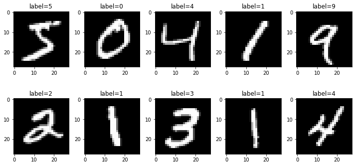
(1) 70000개의 이미지중 0~9에 해당하는 이미지는 각각 몇장씩 들어있는가?
(풀이)
_y = ytrain.tolist()+ytest.tolist(){s:_y.count(s) for s in set(_y)}{0: 6903,
1: 7877,
2: 6990,
3: 7141,
4: 6824,
5: 6313,
6: 6876,
7: 7293,
8: 6825,
9: 6958}(2) \({\tt xtrain}\)에서 손글씨 0을 의미하는 이미지만을 모아서 새로운 텐서 \({\tt xtrain0}\)를 만들어라. 이 텐서에서 처음과 마지막 이미지를 출력하라.
hint: \({\tt xtrain0}\) 의 shape은 (5923,28,28)이어야 한다.
(풀이)
xtrain0 = xtrain[ytrain==0]
xtrain0.shape
(5923, 28, 28)plt.imshow(xtrain0[0],cmap='gray') # 처음이미지<matplotlib.image.AxesImage at 0x7f4574142880>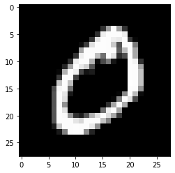
plt.imshow(xtrain0[-1],cmap='gray') # 마지막이미지<matplotlib.image.AxesImage at 0x7f45740b1bb0>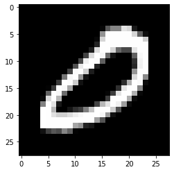
(3) \({\tt xtrain}\)에서 손글씨 0을 의미하는 이미지의 평균을 계산하라. 즉 아래를 계산하라.
- \({\tt xtrain0mean} = \frac{1}{5923}\sum_{i=1}^{5923} {\tt xtrain0[i, :, :]}\)
계산결과를 출력하라.
(풀이)
plt.imshow(xtrain0.mean(axis=0),cmap='gray')<matplotlib.image.AxesImage at 0x7f4573d89a60>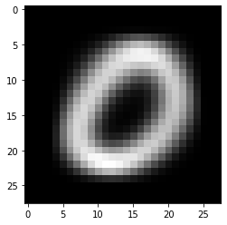
(4) \({\tt xtrain}\)에서 각 라벨에 대한 평균이미지를 계산하고 계산결과를 \({\tt imgmean}\)에 길이가 10인 list로 저장하라. 즉 \({\tt imgmean}\)은 아래와 같은 자료구조를 가지고 있어야 한다.
- \({\tt imgmean}=\big[{\tt imgmean[0]},\dots, {\tt imgmean[9]}\big]\)
- \({\tt imgmean[0]}, \dots, {\tt imgmean[9]}\) 는 각각 (28,28)의 shape을 가진 numpy array
- \({\tt imgmean[0]}, \dots, {\tt imgmean[9]}\) 는 각각 숫자 0,1, …, 9의 평균이미지를 의미
\({\tt imgmean[0]},\dots, {\tt imgmean[9]}\)를 시각화 하라.
(풀이)
imgmean = [xtrain[ytrain==i].mean(axis=0) for i in range(10)] fig, ax = plt.subplots(2,5,figsize=(10,5))
ax[0][0].imshow(imgmean[0],cmap='gray')
ax[0][1].imshow(imgmean[1],cmap='gray')
ax[0][2].imshow(imgmean[2],cmap='gray')
ax[0][3].imshow(imgmean[3],cmap='gray')
ax[0][4].imshow(imgmean[4],cmap='gray')
ax[1][0].imshow(imgmean[5],cmap='gray')
ax[1][1].imshow(imgmean[6],cmap='gray')
ax[1][2].imshow(imgmean[7],cmap='gray')
ax[1][3].imshow(imgmean[8],cmap='gray')
ax[1][4].imshow(imgmean[9],cmap='gray')
fig.tight_layout()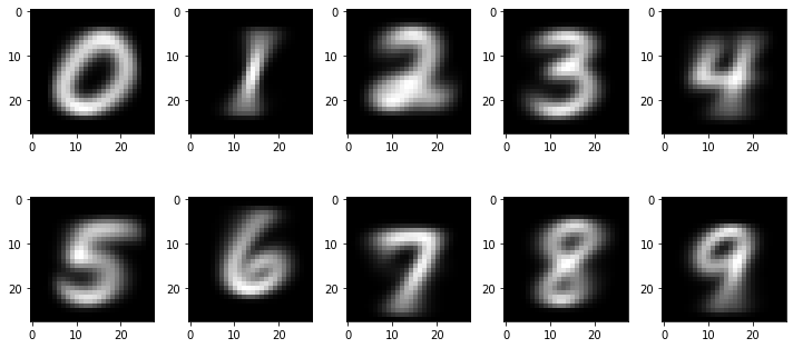
(5) \({\tt xtrain}\)의 두번째 이미지와 \({\tt imgmean[0]}\)의 차이를 제곱한 값의 평균을 구하라. 즉 아래를 계산하라.
- \(\frac{1}{28\times 28} \sum_{p=0}^{27}\sum_{q=0}^{27}\big({\tt xtrain[1,p,q]}-{\tt imgmean[0][p,q]}\big)^2\)
(풀이)
np.mean((xtrain[1,:,:]- imgmean[0])**2)2299.9585279846365(6) 모든 \(j=0,1,\dots,9\) 에 대하여 아래를 계산하라.
- \(\frac{1}{28\times 28} \sum_{p=0}^{27}\sum_{q=0}^{27}\big({\tt xtrain[1,p,q]}-{\tt imgmean[j][p,q]}\big)^2\)
계산값이 가장 작게 나오는 \(j\)는 얼마인가? 위의 계산결과를 토대로 \({\tt xtrain}\)의 두번째 이미지는 어떠한 숫자를 의미한다고 “분류”하는 것이 타당한가?
[np.mean((xtrain[1,:,:]- imgmean[i])**2) for i in range(10)][2299.9585279846365,
7474.876421640121,
6154.997099653264,
5889.84882305034,
6763.709480023399,
4616.900123430389,
5856.367892213506,
6465.999476962735,
5916.546346421647,
6385.5252510342525](7) 아래와 같은 numpy array 를 생성하라.
\[{\tt loss}= \begin{bmatrix} {\tt loss[0,0]} & \dots & {\tt loss[0,9]} \\ {\tt loss[1,0]} & \dots & {\tt loss[1,9]} \\ \dots & \dots & \dots \\ {\tt loss[59999,0]}& \dots &{\tt loss[59999,9]} \\ \end{bmatrix}\]
단, \({\tt loss[i,j]} = \frac{1}{28\times 28} \sum_{p=0}^{27}\sum_{q=0}^{27}\big({\tt xtrain[i,p,q]}-{\tt imgmean[j][p,q]}\big)^2\)
위에서 생성한 \({\tt loss}\)를 이용해 (6)와 같은 방식으로 \({\tt xtrain}\)의 모든 이미지에 대한 분류를 수행하라.
hint: \({\tt loss}\)에서 “최소값을 가지는 원소의 인덱스를 출력”하는 함수를 각 행별로 적용하면 된다.
(풀이)
loss = np.array([[np.mean((xtrain[j,:,:]- imgmean[i])**2) for i in range(10)] for j in range(60000)])loss.argmin(axis=1)array([5, 0, 4, ..., 5, 6, 8])(8) (7)에서 수행한 분류결과와 실제 라벨 \({\tt ytrain}\)을 비교하라. 얼마나 많은 결과가 일치하는지 비율을 계산하라.
(풀이)
np.sum(ytrain == loss.argmin(axis=1)) / 600000.8079833333333334(9) \({\tt xtrain}\)에서 학습한 평균이미지 \({\tt imgmean}\)를 바탕으로 \({\tt xtest}\)의 이미지를 분류하라. 분류결과를 \({\tt ytest}\)와 비교하라. 얼마나 많은 결과가 일치하는지 비율을 계산하라.
(풀이)
est = np.array([[np.mean((xtest[j,:,:]- imgmean[i])**2) for i in range(10)] for j in range(10000)]).argmin(axis=1)np.sum(est == ytest)/100000.8203(10) (9)의 과정에서 잘못분류된 이미지 10개를 선택하여 시각화 하라.
- 실제 라벨과 잘못된 라벨을 구분하여 시각화 할 것
_ytest = ytest[est != ytest]
_xtest = xtest[est != ytest]
_est = est[est != ytest]
fig, ax = plt.subplots(2,5,figsize=(10,5))
ax[0][0].imshow(_xtest[0],cmap='gray'); ax[0][0].set_title('{}/{}'.format(_ytest[0],_est[0]));
ax[0][1].imshow(_xtest[1],cmap='gray'); ax[0][1].set_title('{}/{}'.format(_ytest[1],_est[1]));
ax[0][2].imshow(_xtest[2],cmap='gray'); ax[0][2].set_title('{}/{}'.format(_ytest[2],_est[2]));
ax[0][3].imshow(_xtest[3],cmap='gray'); ax[0][3].set_title('{}/{}'.format(_ytest[3],_est[3]));
ax[0][4].imshow(_xtest[4],cmap='gray'); ax[0][4].set_title('{}/{}'.format(_ytest[4],_est[4]));
ax[1][0].imshow(_xtest[5],cmap='gray'); ax[1][0].set_title('{}/{}'.format(_ytest[5],_est[5]));
ax[1][1].imshow(_xtest[6],cmap='gray'); ax[1][1].set_title('{}/{}'.format(_ytest[6],_est[6]));
ax[1][2].imshow(_xtest[7],cmap='gray'); ax[1][2].set_title('{}/{}'.format(_ytest[7],_est[7]));
ax[1][3].imshow(_xtest[8],cmap='gray'); ax[1][3].set_title('{}/{}'.format(_ytest[8],_est[8]));
ax[1][4].imshow(_xtest[9],cmap='gray'); ax[1][4].set_title('{}/{}'.format(_ytest[9],_est[9]));
fig.tight_layout()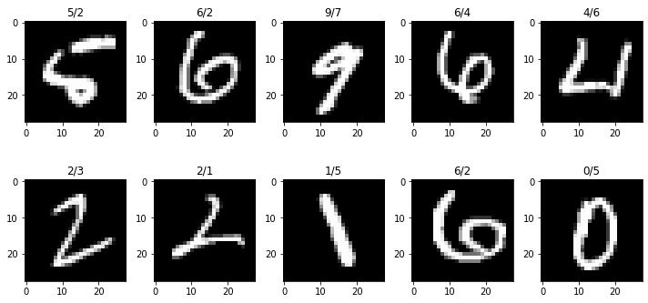
FIFA23 자료분석
아래는 FIFA23 자료를 불러오는 코드이다.
df=pd.read_csv('https://raw.githubusercontent.com/guebin/DV2022/master/posts/FIFA23_official_data.csv').drop(columns=['Loaned From', 'Best Overall Rating']).dropna()
df.head()| ID | Name | Age | Photo | Nationality | Flag | Overall | Potential | Club | Club Logo | ... | Work Rate | Body Type | Real Face | Position | Joined | Contract Valid Until | Height | Weight | Release Clause | Kit Number | |
|---|---|---|---|---|---|---|---|---|---|---|---|---|---|---|---|---|---|---|---|---|---|
| 0 | 209658 | L. Goretzka | 27 | https://cdn.sofifa.net/players/209/658/23_60.png | Germany | https://cdn.sofifa.net/flags/de.png | 87 | 88 | FC Bayern München | https://cdn.sofifa.net/teams/21/30.png | ... | High/ Medium | Unique | Yes | <span class="pos pos28">SUB | Jul 1, 2018 | 2026 | 189cm | 82kg | €157M | 8.0 |
| 1 | 212198 | Bruno Fernandes | 27 | https://cdn.sofifa.net/players/212/198/23_60.png | Portugal | https://cdn.sofifa.net/flags/pt.png | 86 | 87 | Manchester United | https://cdn.sofifa.net/teams/11/30.png | ... | High/ High | Unique | Yes | <span class="pos pos15">LCM | Jan 30, 2020 | 2026 | 179cm | 69kg | €155M | 8.0 |
| 2 | 224334 | M. Acuña | 30 | https://cdn.sofifa.net/players/224/334/23_60.png | Argentina | https://cdn.sofifa.net/flags/ar.png | 85 | 85 | Sevilla FC | https://cdn.sofifa.net/teams/481/30.png | ... | High/ High | Stocky (170-185) | No | <span class="pos pos7">LB | Sep 14, 2020 | 2024 | 172cm | 69kg | €97.7M | 19.0 |
| 3 | 192985 | K. De Bruyne | 31 | https://cdn.sofifa.net/players/192/985/23_60.png | Belgium | https://cdn.sofifa.net/flags/be.png | 91 | 91 | Manchester City | https://cdn.sofifa.net/teams/10/30.png | ... | High/ High | Unique | Yes | <span class="pos pos13">RCM | Aug 30, 2015 | 2025 | 181cm | 70kg | €198.9M | 17.0 |
| 4 | 224232 | N. Barella | 25 | https://cdn.sofifa.net/players/224/232/23_60.png | Italy | https://cdn.sofifa.net/flags/it.png | 86 | 89 | Inter | https://cdn.sofifa.net/teams/44/30.png | ... | High/ High | Normal (170-) | Yes | <span class="pos pos13">RCM | Sep 1, 2020 | 2026 | 172cm | 68kg | €154.4M | 23.0 |
5 rows × 27 columns
(1) 선수들의 평균임금(Wage)을 구하라.
삼성전자와 SK하이닉스
아래는 삼성전자와 SK하이닉스의 주가를 load하는 코드이다.
import yfinance as yf

# 삼성전자와 SK하이닉스의 종목 코드
tickers = ["005930.KS", "017670.KS"]

# 주가 데이터를 불러올 기간
start_date = "2021-01-01"
end_date = "2023-05-02"

# yfinance를 이용하여 데이터 다운로드
df = yf.download(tickers, start=start_date, end=end_date)['Adj Close']
df.columns = pd.Index(['삼성전자','SKT'])

# 데이터 확인
df
[*********************100%***********************] 2 of 2 completed| 삼성전자 | SKT | |
|---|---|---|
| Date | ||
| 2021-01-04 | 79093.812500 | 69000.554688 |
| 2021-01-05 | 79951.445312 | 71620.828125 |
| 2021-01-06 | 78331.453125 | 72930.960938 |
| 2021-01-07 | 78998.507812 | 78608.226562 |
| 2021-01-08 | 84620.843750 | 77152.507812 |
| ... | ... | ... |
| 2023-04-24 | 65200.000000 | 47700.000000 |
| 2023-04-25 | 63600.000000 | 47750.000000 |
| 2023-04-26 | 64100.000000 | 47500.000000 |
| 2023-04-27 | 64600.000000 | 47350.000000 |
| 2023-04-28 | 65500.000000 | 47700.000000 |
574 rows × 2 columns