10/06: [딥러닝의 기초] 깊은신경망(2)
시벤코정리, MNIST with DNN
강의영상
youtube: https://youtube.com/playlist?list=PLQqh36zP38-x9XuXWwAmKKI3JbTRoXVJA
imports
시벤코정리
지난시간 논리전개
- 아이디어: linear -> relu -> linear (-> sigmoid) 조합으로 꺽은선으로 표현되는 underlying 을 표현할 수 있었다. - 아이디어의 실용성: 실제자료에서 꺽은선으로 표현되는 underlying은 몇개 없을 것 같음. 그건 맞는데 꺽이는 점을 많이 설정하면 얼추 비슷하게는 “근사” 시킬 수 있음. - 아이디어의 확장성: 이러한 논리전개는 X:(n,2)인 경우도 가능했음. (이 경우 꺽인선은 꺽인평면이 된다) - 아이디어에 해당하는 용어정리: : 이 구조가 x->y 로 바로 가는 것이 아니라 x->(u1->v1)->(u2->v2)=y 의 구조인데 이러한 네트워크를 하나의 은닉층을 포함하는 네트워크라고 표현한다.
시벤코정리
universal approximation thm: (범용근사정리,보편근사정리,시벤코정리), 1989
하나의 은닉층을 가지는 “linear -> sigmoid -> linear” 꼴의 네트워크를 이용하여 세상에 존재하는 모든 (다차원) 연속함수를 원하는 정확도로 근사시킬 수 있다. (계수를 잘 추정한다면)
- 사실 엄청 이해안되는 정리임. 왜냐햐면, - 그렇게 잘 맞추면 1989년에 세상의 모든 문제를 다 풀어야 한거 아니야? - 요즘은 “linear -> sigmoid -> linear” 가 아니라 “linear -> relu -> linear” 조합으로 많이 쓰던데? - 요즘은 하나의 은닉층을 포함하는 네트워크는 잘 안쓰지 않나? 은닉층이 여러개일수록 좋다고 어디서 본 것 같은데?
- 약간의 의구심이 있지만 아무튼 universal approximation thm에 따르면 우리는 아래와 같은 무기를 가진 꼴이 된다. - 우리의 무기: \({\bf X}: (n,p)\) 꼴의 입력에서 \({\bf y}:(n,1)\) 꼴의 출력으로 향하는 맵핑을 “linear -> relu -> linear”와 같은 네트워크를 이용해서 “근사”시킬 수 있다.
MNIST with DNN
목표
- 목표: \({\bf X}:(n,1,28,28)\) 에서 \(y:(n,1)\) 로 가는 맵핑을 학습하자 –> 배운적이 없는데? –> \({\bf X}:(n,784)\) 에서 \(y:(n,1)\) 로 가는 맵핑을 학습하자..
예비학습1: Path
- path 도 오브젝트임
- path 도 정보+기능이 있음
- path의 정보
- 기능1
(#2) [Path('/home/cgb4/.fastai/data/mnist_png/training'),Path('/home/cgb4/.fastai/data/mnist_png/testing')]- 기능2
- 기능1과 기능2의 결합
(#6131) [Path('/home/cgb4/.fastai/data/mnist_png/training/3/37912.png'),Path('/home/cgb4/.fastai/data/mnist_png/training/3/12933.png'),Path('/home/cgb4/.fastai/data/mnist_png/training/3/3576.png'),Path('/home/cgb4/.fastai/data/mnist_png/training/3/59955.png'),Path('/home/cgb4/.fastai/data/mnist_png/training/3/23144.png'),Path('/home/cgb4/.fastai/data/mnist_png/training/3/40836.png'),Path('/home/cgb4/.fastai/data/mnist_png/training/3/25536.png'),Path('/home/cgb4/.fastai/data/mnist_png/training/3/42669.png'),Path('/home/cgb4/.fastai/data/mnist_png/training/3/7046.png'),Path('/home/cgb4/.fastai/data/mnist_png/training/3/47380.png')...]- ‘/home/cgb4/.fastai/data/mnist_png/training/3/37912.png’ 이 파일을 더블클릭하면 이미지가 보인단 말임
예비학습2: plt.imshow
예비학습3: torchvision
- ’/home/cgb4/.fastai/data/mnist_png/training/3/37912.png’의 이미지파일을 torchvision.io.read_image 를 이용하여 텐서로 만듬
tensor([[[  0,   0,   0,   0,   0,   0,   0,   0,   0,   0,   0,   0,   0,   0,
            0,   0,   0,   0,   0,   0,   0,   0,   0,   0,   0,   0,   0,   0],
         [  0,   0,   0,   0,   0,   0,   0,   0,   0,   0,   0,   0,   0,   0,
            0,   0,   0,   0,   0,   0,   0,   0,   0,   0,   0,   0,   0,   0],
         [  0,   0,   0,   0,   0,   0,   0,   0,   0,   0,   0,   0,   0,   0,
            0,   0,   0,   0,   0,   0,   0,   0,   0,   0,   0,   0,   0,   0],
         [  0,   0,   0,   0,   0,   0,   0,   0,   0,   0,   0,   0,   0,   0,
            0,   0,   0,   0,   0,   0,   0,   0,   0,   0,   0,   0,   0,   0],
         [  0,   0,   0,   0,   0,   0,   0,   0,   0,   0,   0,   0,   0,   0,
            0,   0,   0,   0,   0,   0,   0,   0,   0,   0,   0,   0,   0,   0],
         [  0,   0,   0,   0,   0,   0,   0,   0,   0,   0,   0,  17,  66, 138,
          149, 180, 138, 138,  86,   0,   0,   0,   0,   0,   0,   0,   0,   0],
         [  0,   0,   0,   0,   0,   0,   0,   0,  22, 162, 161, 228, 252, 252,
          253, 252, 252, 252, 252,  74,   0,   0,   0,   0,   0,   0,   0,   0],
         [  0,   0,   0,   0,   0,   0,   0,   0, 116, 253, 252, 252, 252, 189,
          184, 110, 119, 252, 252,  32,   0,   0,   0,   0,   0,   0,   0,   0],
         [  0,   0,   0,   0,   0,   0,   0,   0,  74, 161, 160,  77,  45,   4,
            0,   0,  70, 252, 210,   0,   0,   0,   0,   0,   0,   0,   0,   0],
         [  0,   0,   0,   0,   0,   0,   0,   0,   0,   0,   0,   0,   0,   0,
            0,  22, 205, 252,  32,   0,   0,   0,   0,   0,   0,   0,   0,   0],
         [  0,   0,   0,   0,   0,   0,   0,   0,   0,   0,   0,   0,   0,   0,
            0, 162, 253, 245,  21,   0,   0,   0,   0,   0,   0,   0,   0,   0],
         [  0,   0,   0,   0,   0,   0,   0,   0,   0,   0,   0,   0,   0,   0,
           36, 219, 252, 139,   0,   0,   0,   0,   0,   0,   0,   0,   0,   0],
         [  0,   0,   0,   0,   0,   0,   0,   0,   0,   0,   0,   0,   0,   0,
          222, 252, 202,  13,   0,   0,   0,   0,   0,   0,   0,   0,   0,   0],
         [  0,   0,   0,   0,   0,   0,   0,   0,   0,   0,   0,   0,   0,  43,
          253, 252,  89,   0,   0,   0,   0,   0,   0,   0,   0,   0,   0,   0],
         [  0,   0,   0,   0,   0,   0,   0,   0,   0,   0,   0,   0,  85, 240,
          253, 157,   6,   0,   0,   0,   0,   0,   0,   0,   0,   0,   0,   0],
         [  0,   0,   0,   0,   0,   0,   0,   0,   0,   0,   0,   7, 160, 253,
          231,  42,   0,   0,   0,   0,   0,   0,   0,   0,   0,   0,   0,   0],
         [  0,   0,   0,   0,   0,   0,   0,   0,   0,   0,   0, 142, 252, 252,
           42,  30,  78, 161,  36,   0,   0,   0,   0,   0,   0,   0,   0,   0],
         [  0,   0,   0,   0,   0,   0,   0,   0,   0,   0,   0, 184, 252, 252,
          185, 228, 252, 252, 168,   0,   0,   0,   0,   0,   0,   0,   0,   0],
         [  0,   0,   0,   0,   0,   0,   0,   0,   0,   0,   0, 184, 252, 252,
          253, 252, 252, 252, 116,   0,   0,   0,   0,   0,   0,   0,   0,   0],
         [  0,   0,   0,   0,   0,   0,   0,   0,   0,   0,   0, 101, 179, 252,
          253, 252, 252, 210,  12,   0,   0,   0,   0,   0,   0,   0,   0,   0],
         [  0,   0,   0,   0,   0,   0,   0,   0,   0,   0,   0,   0,   0,  22,
          255, 253, 215,  21,   0,   0,   0,   0,   0,   0,   0,   0,   0,   0],
         [  0,   0,   0,   0,   0,   0,   0,   0,   0,   0,   0,  34,  89, 244,
          253, 223,  98,   0,   0,   0,   0,   0,   0,   0,   0,   0,   0,   0],
         [  0,   0,   0,   0,   0,   0,   0,   0, 116, 123, 142, 234, 252, 252,
          184,  67,   0,   0,   0,   0,   0,   0,   0,   0,   0,   0,   0,   0],
         [  0,   0,   0,   0,   0,   0,   0,   0, 230, 253, 252, 252, 252, 168,
            0,   0,   0,   0,   0,   0,   0,   0,   0,   0,   0,   0,   0,   0],
         [  0,   0,   0,   0,   0,   0,   0,   0, 126, 253, 252, 168,  43,   2,
            0,   0,   0,   0,   0,   0,   0,   0,   0,   0,   0,   0,   0,   0],
         [  0,   0,   0,   0,   0,   0,   0,   0,   0,   0,   0,   0,   0,   0,
            0,   0,   0,   0,   0,   0,   0,   0,   0,   0,   0,   0,   0,   0],
         [  0,   0,   0,   0,   0,   0,   0,   0,   0,   0,   0,   0,   0,   0,
            0,   0,   0,   0,   0,   0,   0,   0,   0,   0,   0,   0,   0,   0],
         [  0,   0,   0,   0,   0,   0,   0,   0,   0,   0,   0,   0,   0,   0,
            0,   0,   0,   0,   0,   0,   0,   0,   0,   0,   0,   0,   0,   0]]],
       dtype=torch.uint8)
- 이 텐서는 (1,28,28)의 shape을 가짐
- imgtsr를 plt.imshow 로 시각화
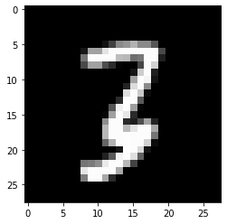
- 진짜 숫자3이 있음
데이터정리
(6131, 6265)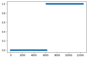
- “y=0”은 숫자3을 의미, “y=1”은 숫자7을 의미
- 숫자3은 6131개, 숫자7은 6265개 있음
학습 (숙제: 스스로 확인해 볼 것)
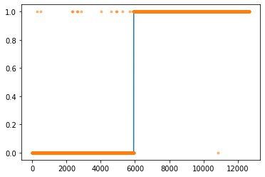
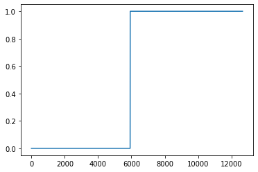
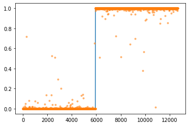
- 네트워크의 설계
- \(\underset{(n,784)}{\bf X} \overset{l_1}{\to} \underset{(n,30)}{\boldsymbol u^{(1)}} \overset{a_1}{\to} \underset{(n,30)}{\boldsymbol v^{(1)}} \overset{l_1}{\to} \underset{(n,1)}{\boldsymbol u^{(2)}} \overset{a_2}{\to} \underset{(n,1)}{\boldsymbol v^{(2)}}=\underset{(n,1)}{\hat{\boldsymbol y}}\)
- 대부분 잘 적합되었음
숙제
youtube: https://youtube.com/playlist?list=PLQqh36zP38-zEUnVaQveVvRD-eMBPtxIp
- 숫자0과 숫자1을 구분하는 네트워크를 아래와 같은 구조로 설계하라
\[\underset{(n,784)}{\bf X} \overset{l_1}{\to} \underset{(n,64)}{\boldsymbol u^{(1)}} \overset{a_1}{\to} \underset{(n,64)}{\boldsymbol v^{(1)}} \overset{l_1}{\to} \underset{(n,1)}{\boldsymbol u^{(2)}} \overset{a_2}{\to} \underset{(n,1)}{\boldsymbol v^{(2)}}=\underset{(n,1)}{\hat{\boldsymbol y}}\]
위에서 \(a_1\)은 relu를, \(a_2\)는 sigmoid를 의미한다.
- “y=0”은 숫자0을 의미하도록 하고 “y=1”은 숫자1을 의미하도록 설정하라.
(풀이)
X0 = torch.stack([torchvision.io.read_image(str(fname)) for fname in (path/'training/0').ls()])
X1 = torch.stack([torchvision.io.read_image(str(fname)) for fname in (path/'training/1').ls()])
X = torch.concat([X0,X1]).reshape(-1,1*28*28).float()
y = torch.tensor([0.0]*len(X0) + [1.0]*len(X1)).reshape(-1,1)- 아래의 지침에 따라 200 epoch 학습을 진행하라.
- 손실함수는 BECLoss를 이용할 것. torch.nn.BCELoss() 를 이용할 것.
- 옵티마이저는 아담으로 설정할 것. 학습률은 lr=0.002로 설정할 것.
(풀이)
- 아래의 지침에 따라 200 epoch 학습을 진행하라. 학습이 잘 되는가?
- 손실함수는 BECLoss를 이용할 것. torch.nn.BCELoss()를 사용하지 않고 수식을 직접 입력할 것.
- 옵티마이저는 아담으로 설정할 것. 학습률은 lr=0.002로 설정할 것.
(풀이)
- 학습이 잘 안되었다!
- 아래의 지침에 따라 200 epoch 학습을 진행하라. 학습이 잘 되는가?
- 이미지의 값을 0과 1사이로 규격화 하라. (Xnp = Xnp/255 를 이용하세요!)
- 손실함수는 BECLoss를 이용할 것. torch.nn.BCELoss()를 사용하지 않고 수식을 직접 입력할 것.
- 옵티마이저는 아담으로 설정할 것. 학습률은 lr=0.002로 설정할 것.
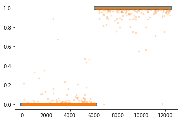
- 이번엔 학습이 잘 되었다!
- 아래와 같은 수식을 이용하여 accuracy를 계산하라.
\(\text{accuracy}=\frac{1}{n}\sum_{i=1}^n I(\tilde{y}_i=y_i)\) - \(\tilde{y}_i = \begin{cases} 1 & \hat{y}_i > 0.5 \\ 0 & \hat{y}_i \leq 0.5 \end{cases}\) - \(I(\tilde{y}_i=y_i) = \begin{cases} 1 & \tilde{y}_i=y_i \\ 0 & \tilde{y}_i \neq y_i \end{cases}\)
단, \(n\)은 0과 1을 의미하는 이미지의 수
(풀이1)
- \(\tilde{y}_i = \begin{cases} 1 & \hat{y}_i > 0.5 \\ 0 & \hat{y}_i \leq 0.5 \end{cases}\) 의 구현
- \(I(\tilde{y}_i=y_i) = \begin{cases} 1 & \tilde{y}_i=y_i \\ 0 & \tilde{y}_i \neq y_i \end{cases}\) 의 구현
- \(\sum_{i=1}^n I(\tilde{y}_i=y_i)\)의 계산
- \(\text{accuracy}=\frac{1}{n}\sum_{i=1}^n I(\tilde{y}_i=y_i)\) 의 계산
(풀이2)
생각해볼점1: 왜 (2)는 학습이 잘되고 (3)은 학습이 잘 안되는가?
- data
X0 = torch.stack([torchvision.io.read_image(str(fname)) for fname in (path/'training/0').ls()])
X1 = torch.stack([torchvision.io.read_image(str(fname)) for fname in (path/'training/1').ls()])
X = torch.concat([X0,X1]).reshape(-1,1*28*28).float()
y = torch.tensor([0.0]*len(X0) + [1.0]*len(X1)).reshape(-1,1)
- net초기화
- loss_fn 정의
- loss_fn 적용결과 확인
(tensor(22.4927, grad_fn=<BinaryCrossEntropyBackward0>),
tensor(nan, grad_fn=<NegBackward0>))- loss_fn1(net(x),y) = 22.4927
- loss_fn2(net(x),y) = nan (해설영상에는 \(\infty\)라고 했는데 정확하게는 nan입니다. nan은 \(\infty \times 0\)의 결과로 나오게 되고요 \(y_i=1,\hat{y}_i=1\) 인 경우에 \(-\frac{1}{n}\sum_{i=1}^{n}\big(y_i\log(\hat{y}_i) + (1-y_i)\log(1-\hat{y}_i)\big)\) 중 \((1-y_i)\log(1-\hat{y}_i)\)의 계산결과로 발생할 수 있습니다.)
- 왜?
- 처음 4개의 관측치에 대한 loss_fn 적용 결과: 같다.
(tensor(3.0566, grad_fn=<BinaryCrossEntropyBackward0>),
 tensor(3.0566, grad_fn=<NegBackward0>))
- 처음 5개의 관측치에 대한 loss_fn 적용 결과: 다르다.
(tensor(22.4453, grad_fn=<BinaryCrossEntropyBackward0>),
 tensor(inf, grad_fn=<NegBackward0>))
- 왜? 5번관측치에 문제가 있음
(tensor([[1.2304e-02],
         [9.9999e-01],
         [4.5096e-09],
         [4.0554e-01],
         [1.0000e+00]], grad_fn=<SliceBackward0>),
 tensor([[0.],
         [0.],
         [0.],
         [0.],
[0.]]))(tensor(100., grad_fn=<BinaryCrossEntropyBackward0>),
tensor(inf, grad_fn=<NegBackward0>))- loss_fn1은 사실 이런식으로 계산을 했음
- loss function에 대한 엄밀한 정의는 아닌데 \(\infty =100\) 으로 생각하는 것이 오히려 효율적이다.
생각해볼점2: 왜 (3)은 학습이 잘 안되는데 (4)는 학습이 잘 되는가?
- 아래의 상황을 다시 생각하자.
X0 = torch.stack([torchvision.io.read_image(str(fname)) for fname in (path/'training/0').ls()])
X1 = torch.stack([torchvision.io.read_image(str(fname)) for fname in (path/'training/1').ls()])
X = torch.concat([X0,X1]).reshape(-1,1*28*28).float()
y = torch.tensor([0.0]*len(X0) + [1.0]*len(X1)).reshape(-1,1)- (3)에서 학습이 불가능했던 만악의 근원은 \(y=0\) 인데 \(yhat \approx 1\) 인 상황 이었다. (\(y=1\)인데 \(yhat \approx 0\) 인 상황도 마찬가지) - 그런데 왜 초기값에 \(yhat\approx 1\) 과 같은 값이 들어있는 거야?
- 네트워크를 분해하자.
- 5번관측치 X[[5]]를 콕 찍어서 생각해보자.
- 만약에 하나의 관측치 X[[5]]의 범위를 0~1 사이로 맞춘다면?
(tensor(inf, grad_fn=<NegBackward0>), tensor(0.7558, grad_fn=<NegBackward0>))- 깨달음1 - X가 0~255사이의 값을 가지면 \(X \to u^{(1)} \to v^{(1)} \to u^{(2)} \to yhat\) 의 구조에서 \(u^{(2)}\)의 값이 클 확률이 높다. (예를들면 21.7626 같은 값) - 큰 \(u^{(2)}\)의 값은 \(yhat \approx 1\) 이 되는 상황을 야기한다. - \(yhat \approx 1\)인 상황은 \(loss=\infty\)인 상황을 야기한다. - 그래서 학습이 안된다.
- 깨달음2 - X가 0~1사이의 값을 가지면 \(X \to u^{(1)} \to v^{(1)} \to u^{(2)} \to yhat\) 의 구조에서 \(u^{(2)}\)의 값이 클 확률이 적다. (예를들면 0.1216와 같이 적당한 값이 나옴) - 적당한 크기의 \(u^{(2)}\)의 값은 \(yhat \approx 1\) 이 되는 상황을 만들지 않는다. - 그래서 \(loss=\infty\)인 상황도 잘 생기지 않는다. - 그래서 학습이 (상대적으로) 잘된다.