11wk-1: 순환신경망 (4)

순환신경망
Author

최규빈

Published

November 10, 2022

11/10: [순환신경망] RNN (2)

AbAcAd예제(3)

강의영상

youtube: https://youtube.com/playlist?list=PLQqh36zP38-zRWSBjuvzsjPe6JxnHO4AX

import

import torch
import numpy as np
import matplotlib.pyplot as plt

Define some funtions
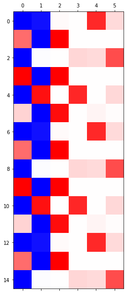
def f(txt,mapping):
    return [mapping[key] for key in txt] 
soft = torch.nn.Softmax(dim=1)

Exam4: AbAcAd (3)

data

- 기존의 정리방식

txt = list('AbAcAd')*100
txt[:10]
['A', 'b', 'A', 'c', 'A', 'd', 'A', 'b', 'A', 'c']
txt_x = txt[:-1]
txt_y = txt[1:]
txt_x[:5],txt_y[:5]
(['A', 'b', 'A', 'c', 'A'], ['b', 'A', 'c', 'A', 'd'])
x = torch.nn.functional.one_hot(torch.tensor(f(txt_x,{'A':0,'b':1,'c':2,'d':3}))).float()
y = torch.nn.functional.one_hot(torch.tensor(f(txt_y,{'A':0,'b':1,'c':2,'d':3}))).float()
x,y
(tensor([[1., 0., 0., 0.],
         [0., 1., 0., 0.],
         [1., 0., 0., 0.],
         ...,
         [1., 0., 0., 0.],
         [0., 0., 1., 0.],
         [1., 0., 0., 0.]]),
 tensor([[0., 1., 0., 0.],
         [1., 0., 0., 0.],
         [0., 0., 1., 0.],
         ...,
         [0., 0., 1., 0.],
         [1., 0., 0., 0.],
         [0., 0., 0., 1.]]))

순환신경망 구현2 (with RNNCell, hidden node 2)

ref: https://pytorch.org/docs/stable/generated/torch.nn.RNNCell.html

(1) 숙성네트워크

torch.manual_seed(43052)
rnncell = torch.nn.RNNCell(4,2) # x:(n,4) h:(n,2) 

(2) 조리네트워크

torch.manual_seed(43052)
cook = torch.nn.Linear(2,4) # 숙성된 2차원의 단어를 다시 4차원으로 바꿔줘야지 나중에 softmax취할 수 있음

(3) 손실함수와 옵티마이저

loss_fn = torch.nn.CrossEntropyLoss()
optimizr = torch.optim.Adam(list(rnncell.parameters())+list(cook.parameters()))

(4) 학습

T = len(x) 
for epoc in range(5000):
    ## 1~2
    loss = 0 
    ht = torch.zeros(1,2) 
    for t in range(T):
        xt,yt = x[[t]], y[[t]]
        ht = rnncell(xt,ht)
        ot = cook(ht)
        loss = loss + loss_fn(ot,yt) 
    ## 3 
    loss.backward()
    ## 4 
    optimizr.step()
    optimizr.zero_grad()

(5) 시각화

hidden = torch.zeros(T,2) 
# t=0 
_water = torch.zeros(1,2)
hidden[[0]] = rnncell(x[[0]],_water)
# t=1~T 
for t in range(1,T):
    hidden[[t]] = rnncell(x[[t]],hidden[[t-1]])
yhat = soft(cook(hidden))
yhat
tensor([[1.9725e-02, 1.5469e-03, 8.2766e-01, 1.5106e-01],
        [9.1875e-01, 1.6513e-04, 6.7702e-02, 1.3384e-02],
        [2.0031e-02, 1.0660e-03, 8.5248e-01, 1.2642e-01],
        ...,
        [1.9640e-02, 1.3568e-03, 8.3705e-01, 1.4196e-01],
        [9.9564e-01, 1.3114e-05, 3.5069e-03, 8.4108e-04],
        [3.5473e-03, 1.5670e-01, 1.4102e-01, 6.9873e-01]],
       grad_fn=<SoftmaxBackward0>)
plt.matshow(yhat[:15].data,cmap='bwr')
<matplotlib.image.AxesImage at 0x7fe67cda0910>

plt.matshow(yhat[-15:].data,cmap='bwr')
<matplotlib.image.AxesImage at 0x7fe67c28ff90>

순환신경망 구현3 (with RNN, hidden node 2) – 성공

(예비학습)

- 네트워크학습이후 yhat을 구하려면 번거로웠음

hidden = torch.zeros(T,2) 
_water = torch.zeros(1,2)
hidden[[0]] = rnncell(x[[0]],_water)
for t in range(1,T):
    hidden[[t]] = rnncell(x[[t]],hidden[[t-1]])
yhat = soft(cook(hidden))

- 이렇게 하면 쉽게(?) 구할 수 있음

rnn = torch.nn.RNN(4,2)
rnn.weight_hh_l0.data = rnncell.weight_hh.data 
rnn.weight_ih_l0.data = rnncell.weight_ih.data
rnn.bias_hh_l0.data = rnncell.bias_hh.data
rnn.bias_ih_l0.data = rnncell.bias_ih.data

- rnn(x,_water)의 결과는 (1) 599년치 간장 (2) 599번째 간장 이다

rnn(x,_water), hidden
((tensor([[-0.9912, -0.9117],
          [ 0.0698, -1.0000],
          [-0.9927, -0.9682],
          ...,
          [-0.9935, -0.9315],
          [ 0.5777, -1.0000],
          [-0.9960, -0.0109]], grad_fn=<SqueezeBackward1>),
  tensor([[-0.9960, -0.0109]], grad_fn=<SqueezeBackward1>)),
 tensor([[-0.9912, -0.9117],
         [ 0.0698, -1.0000],
         [-0.9927, -0.9682],
         ...,
         [-0.9935, -0.9315],
         [ 0.5777, -1.0000],
         [-0.9960, -0.0109]], grad_fn=<IndexPutBackward0>))
soft(cook(rnn(x,_water)[0]))
tensor([[1.9725e-02, 1.5469e-03, 8.2766e-01, 1.5106e-01],
        [9.1875e-01, 1.6513e-04, 6.7702e-02, 1.3384e-02],
        [2.0031e-02, 1.0660e-03, 8.5248e-01, 1.2642e-01],
        ...,
        [1.9640e-02, 1.3568e-03, 8.3705e-01, 1.4196e-01],
        [9.9564e-01, 1.3114e-05, 3.5069e-03, 8.4108e-04],
        [3.5473e-03, 1.5670e-01, 1.4102e-01, 6.9873e-01]],
       grad_fn=<SoftmaxBackward0>)

(예비학습결론) torch.nn.RNN(4,2)는 torch.nn.RNNCell(4,2)의 batch 버전이다. (for문이 포함된 버전이다)


torch.nn.RNN(4,2)를 이용하여 구현하자.

(1) 숙성네트워크

선언

rnn = torch.nn.RNN(4,2)

가중치초기화

torch.manual_seed(43052)
_rnncell = torch.nn.RNNCell(4,2)
rnn.weight_hh_l0.data = _rnncell.weight_hh.data 
rnn.weight_ih_l0.data = _rnncell.weight_ih.data
rnn.bias_hh_l0.data = _rnncell.bias_hh.data
rnn.bias_ih_l0.data = _rnncell.bias_ih.data

(2) 조리네트워크

torch.manual_seed(43052)
cook = torch.nn.Linear(2,4) 

(3) 손실함수와 옵티마이저

loss_fn = torch.nn.CrossEntropyLoss()
optimizr = torch.optim.Adam(list(rnn.parameters())+list(cook.parameters()))

(4) 학습

_water = torch.zeros(1,2) 
for epoc in range(5000):
    ## 1 
    hidden,hT = rnn(x,_water)
    output = cook(hidden) 
    ## 2 
    loss = loss_fn(output,y)
    ## 3 
    loss.backward()
    ## 4 
    optimizr.step()
    optimizr.zero_grad()

(5) 시각화1: yhat

yhat = soft(output)
plt.matshow(yhat.data[:15],cmap='bwr')
<matplotlib.image.AxesImage at 0x7fe67c231310>

  • 처음은 좀 틀렸음 ㅎㅎ
plt.matshow(yhat.data[-15:],cmap='bwr')
<matplotlib.image.AxesImage at 0x7fe67c1c5d90>

  • 뒤에는 잘맞음

실전팁: _water 대신에 hT를 대입 (사실 큰 차이는 없음)

rnn(x[:6],_water),rnn(x[:6],hT)
((tensor([[-0.9912, -0.9117],
          [ 0.0698, -1.0000],
          [-0.9927, -0.9682],
          [ 0.5761, -1.0000],
          [-0.9960, -0.0173],
          [ 0.9960, -1.0000]], grad_fn=<SqueezeBackward1>),
  tensor([[ 0.9960, -1.0000]], grad_fn=<SqueezeBackward1>)),
 (tensor([[-0.9713, -1.0000],
          [ 0.0535, -1.0000],
          [-0.9925, -0.9720],
          [ 0.5759, -1.0000],
          [-0.9960, -0.0180],
          [ 0.9960, -1.0000]], grad_fn=<SqueezeBackward1>),
  tensor([[ 0.9960, -1.0000]], grad_fn=<SqueezeBackward1>)))

(6) 시각화2: hidden, yhat

combinded = torch.concat([hidden,yhat],axis=1)
plt.matshow(combinded[-15:].data,cmap='bwr')
<matplotlib.image.AxesImage at 0x7fe67c13b7d0>

  • 히든노드의 해석이 어려움.

순환신경망 구현4 (with RNN, hidden node 3) – 성공

(1) 숙성네트워크~ (2) 조리네트워크

torch.manual_seed(2) #1 
rnn = torch.nn.RNN(4,3) 
cook = torch.nn.Linear(3,4) 

(3) 손실함수와 옵티마이저

loss_fn = torch.nn.CrossEntropyLoss()
optimizr = torch.optim.Adam(list(rnn.parameters())+list(cook.parameters()))

(4) 학습

_water = torch.zeros(1,3) 
for epoc in range(5000):
    ## 1
    hidden,hT = rnn(x,_water) 
    output = cook(hidden) 
    ## 2 
    loss = loss_fn(output,y) 
    ## 3 
    loss.backward()
    ## 4 
    optimizr.step()
    optimizr.zero_grad()

(5) 시각화1: yhat

yhat = soft(output)
plt.matshow(yhat[-15:].data,cmap='bwr')
<matplotlib.image.AxesImage at 0x7fe67c04f550>

(6) 시각화2: hidden, yhat

combinded = torch.concat([hidden,yhat],axis=1)
plt.matshow(combinded[-15:].data,cmap='bwr')
<matplotlib.image.AxesImage at 0x7fe6747ba910>

  • 세번째 히든노드 = 대소문자를 구분
  • 1,2 히든노드 = bcd를 구분

HW: hello 예제

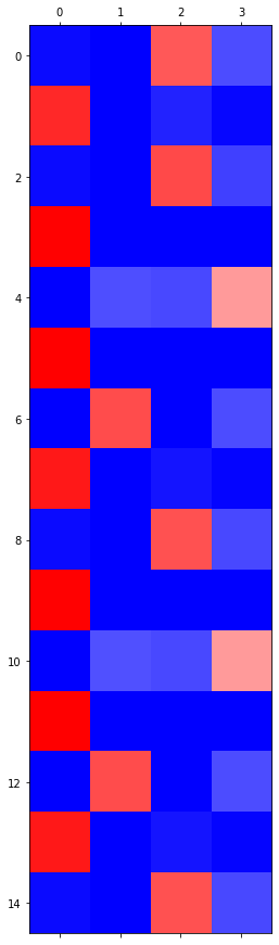
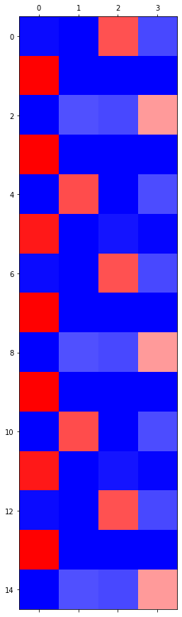
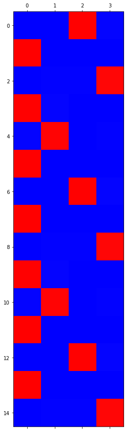
아래와 같이 hello가 반복되는 자료가 있다고 하자.

txt = list('hello')*100
txt[:10]
['h', 'e', 'l', 'l', 'o', 'h', 'e', 'l', 'l', 'o']
txt_x = txt[:-1]
txt_y = txt[1:]
txt_x[:5],txt_y[:5]
(['h', 'e', 'l', 'l', 'o'], ['e', 'l', 'l', 'o', 'h'])
x = torch.nn.functional.one_hot(torch.tensor(f(txt_x,{'h':0,'e':1,'l':2,'o':3}))).float()
y = torch.nn.functional.one_hot(torch.tensor(f(txt_y,{'h':0,'e':1,'l':2,'o':3}))).float()
x,y
(tensor([[1., 0., 0., 0.],
         [0., 1., 0., 0.],
         [0., 0., 1., 0.],
         ...,
         [0., 1., 0., 0.],
         [0., 0., 1., 0.],
         [0., 0., 1., 0.]]),
 tensor([[0., 1., 0., 0.],
         [0., 0., 1., 0.],
         [0., 0., 1., 0.],
         ...,
         [0., 0., 1., 0.],
         [0., 0., 1., 0.],
         [0., 0., 0., 1.]]))

3개의 은닉노드를 가진 RNN을 설계하고 학습시켜라.