11/15: [순환신경망] LSTM (1)
GPU실험, abcabC예제, abcdabcD예제
강의영상
https://youtube.com/playlist?list=PLQqh36zP38-wCXvhHTVOdOLBFD5T5uscl
import
Define some funtions
GPU 실험
실험결과 요약
| len | # of hidden nodes | backward | cpu | gpu | ratio |
|---|---|---|---|---|---|
| 20000 | 20 | O | 93.02 | 3.26 | 28.53 |
| 20000 | 20 | X | 18.85 | 1.29 | 14.61 |
| 2000 | 20 | O | 6.53 | 0.75 | 8.70 |
| 2000 | 20 | X | 1.25 | 0.14 | 8.93 |
| 2000 | 1000 | O | 58.99 | 4.75 | 12.41 |
| 2000 | 1000 | X | 13.16 | 2.29 | 5.74 |
Exam5: abcabC
data
RNN
- 3000 epochs

- 6000 epochs

- 9000 epochs

- 12000 epochs
- 15000 epochs
LSTM
- LSTM
- 3000 epochs
<matplotlib.image.AxesImage at 0x7f47cc0608d0>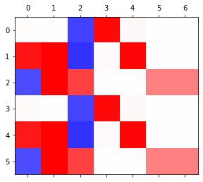
- 6000 epochs
RNN vs LSTM 성능비교실험
- RNN
fig, ax = plt.subplots(5,5,figsize=(10,10))
for i in range(5):
    for j in range(5):
        rnn = torch.nn.RNN(4,3).to("cuda:0")
        linr = torch.nn.Linear(3,4).to("cuda:0")
        loss_fn = torch.nn.CrossEntropyLoss()
        optimizr = torch.optim.Adam(list(rnn.parameters())+list(linr.parameters()),lr=0.1)
        _water = torch.zeros(1,3).to("cuda:0")
        for epoc in range(3000):
            ## 1
            hidden, hT = rnn(x,_water)
            output = linr(hidden)
            ## 2
            loss = loss_fn(output,y)
            ## 3
            loss.backward()
            ## 4
            optimizr.step()
            optimizr.zero_grad()
        yhat=soft(output)
        combind = torch.concat([hidden,yhat],axis=1)
        ax[i][j].matshow(combind.to("cpu").data[-6:],cmap='bwr',vmin=-1,vmax=1)
fig.suptitle(r"$RNN$",size=20)
fig.tight_layout()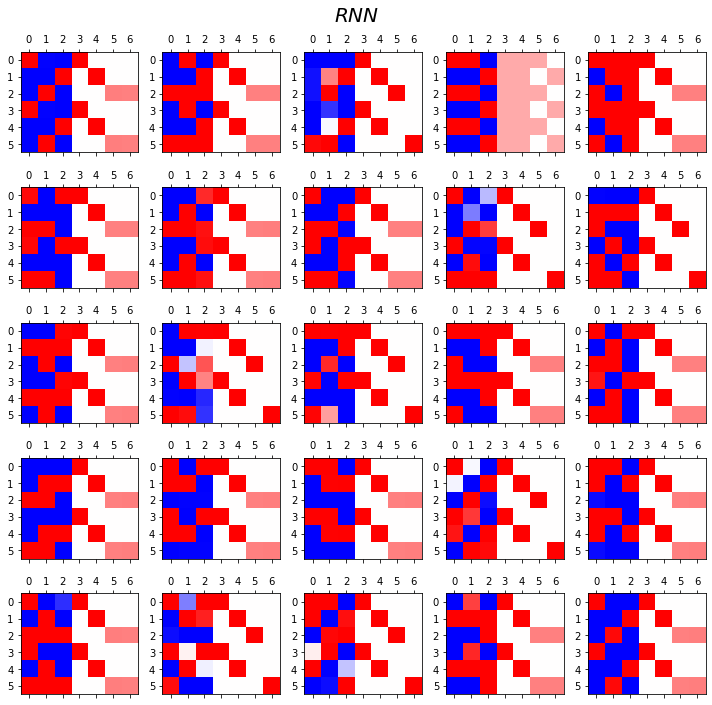
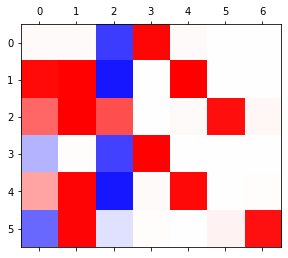
- LSTM
fig, ax = plt.subplots(5,5,figsize=(10,10))
for i in range(5):
    for j in range(5):
        lstm = torch.nn.LSTM(4,3).to("cuda:0")
        linr = torch.nn.Linear(3,4).to("cuda:0")
        loss_fn = torch.nn.CrossEntropyLoss()
        optimizr = torch.optim.Adam(list(lstm.parameters())+list(linr.parameters()),lr=0.1)
        _water = torch.zeros(1,3).to("cuda:0")
        for epoc in range(3000):
            ## 1
            hidden, (hT,cT) = lstm(x,(_water,_water))
            output = linr(hidden)
            ## 2
            loss = loss_fn(output,y)
            ## 3
            loss.backward()
            ## 4
            optimizr.step()
            optimizr.zero_grad()
        yhat=soft(output)
        combind = torch.concat([hidden,yhat],axis=1)
        ax[i][j].matshow(combind.to("cpu").data[-6:],cmap='bwr',vmin=-1,vmax=1)
fig.suptitle(r"$LSTM$",size=20)
fig.tight_layout()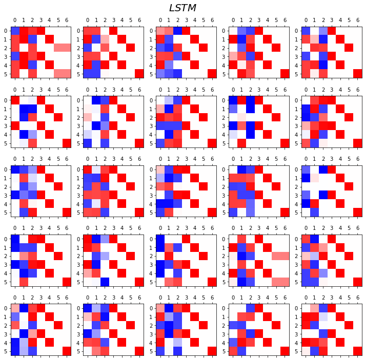
Exam6: abcdabcD
data
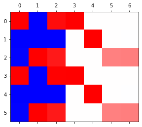
RNN vs LSTM 성능비교실험
- RNN
fig, ax = plt.subplots(5,5,figsize=(10,10))
for i in range(5):
    for j in range(5):
        rnn = torch.nn.RNN(5,4).to("cuda:0")
        linr = torch.nn.Linear(4,5).to("cuda:0")
        loss_fn = torch.nn.CrossEntropyLoss()
        optimizr = torch.optim.Adam(list(rnn.parameters())+list(linr.parameters()),lr=0.1)
        _water = torch.zeros(1,4).to("cuda:0")
        for epoc in range(3000):
            ## 1
            hidden, hT = rnn(x,_water)
            output = linr(hidden)
            ## 2
            loss = loss_fn(output,y)
            ## 3
            loss.backward()
            ## 4
            optimizr.step()
            optimizr.zero_grad()
        yhat=soft(output)
        combind = torch.concat([hidden,yhat],axis=1)
        ax[i][j].matshow(combind.to("cpu").data[-8:],cmap='bwr',vmin=-1,vmax=1)
fig.suptitle(r"$RNN$",size=20)
fig.tight_layout()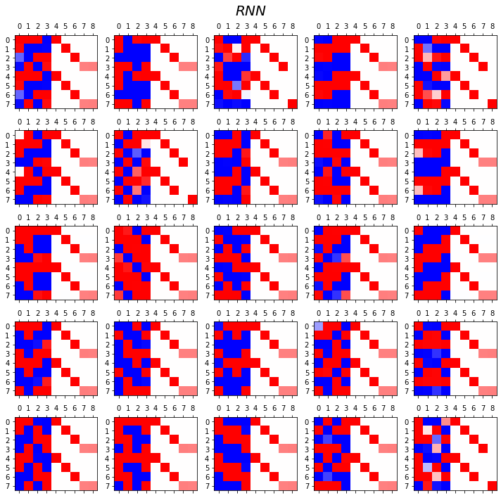
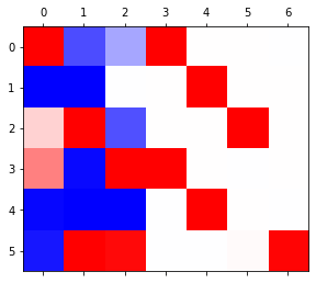
- LSTM
fig, ax = plt.subplots(5,5,figsize=(10,10))
for i in range(5):
    for j in range(5):
        lstm = torch.nn.LSTM(5,4).to("cuda:0")
        linr = torch.nn.Linear(4,5).to("cuda:0")
        loss_fn = torch.nn.CrossEntropyLoss()
        optimizr = torch.optim.Adam(list(lstm.parameters())+list(linr.parameters()),lr=0.1)
        _water = torch.zeros(1,4).to("cuda:0")
        for epoc in range(3000):
            ## 1
            hidden, (hT,cT) = lstm(x,(_water,_water))
            output = linr(hidden)
            ## 2
            loss = loss_fn(output,y)
            ## 3
            loss.backward()
            ## 4
            optimizr.step()
            optimizr.zero_grad()
        yhat=soft(output)
        combind = torch.concat([hidden,yhat],axis=1)
        ax[i][j].matshow(combind.to("cpu").data[-8:],cmap='bwr',vmin=-1,vmax=1)
fig.suptitle(r"$LSTM$",size=20)
fig.tight_layout()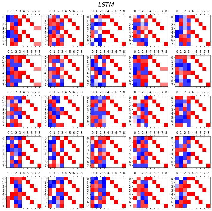
- 관찰1: LSTM이 확실히 장기기억에 강하다.
- 관찰2: LSTM은 hidden에 0이 잘 나온다.
- 사실 확실히 구분되는 특징을 판별할때는 -1,1 로 히든레이어 값들이 설정되면 명확하다.
- 히든레이어에 -1~1사이의 값이 나온다면 애매한 판단이 내려지게 된다.
- 그런데 이 애매한 판단이 어떻게 보면 문맥의 뉘앙스를 이해하는데 더 잘 맞다.
- 그런데 RNN은 -1,1로 셋팅된 상황에서 -1~1로의 변화가 더디다는 것이 문제임.