10wk-2: Plotly – 판다스 백엔드

plotly

Author

최규빈

Published

November 8, 2023

1. 강의영상

2. Imports

import numpy as np
import pandas as pd 
import plotly.io as pio

pd.options.plotting.backend = "plotly"
pio.templates.default = "plotly_white"
print(pio.templates)

Templates configuration
-----------------------
    Default template: 'plotly_white'
    Available templates:
        ['ggplot2', 'seaborn', 'simple_white', 'plotly',
         'plotly_white', 'plotly_dark', 'presentation', 'xgridoff',
         'ygridoff', 'gridon', 'none']

3. 여러가지 플랏

A. `.plot.bar()`

# 예제1 – 성별 합격률 시각화

df = pd.read_csv("https://raw.githubusercontent.com/guebin/DV2022/master/posts/Simpson.csv",index_col=0,header=[0,1]).reset_index().melt(id_vars='index').set_axis(['department','gender','result','count'],axis=1)
df

	department	gender	result	count
0	A	male	fail	314
1	B	male	fail	208
2	C	male	fail	204
3	D	male	fail	279
4	E	male	fail	137
5	F	male	fail	149
6	A	male	pass	511
7	B	male	pass	352
8	C	male	pass	121
9	D	male	pass	138
10	E	male	pass	54
11	F	male	pass	224
12	A	female	fail	19
13	B	female	fail	7
14	C	female	fail	391
15	D	female	fail	244
16	E	female	fail	299
17	F	female	fail	103
18	A	female	pass	89
19	B	female	pass	18
20	C	female	pass	202
21	D	female	pass	131
22	E	female	pass	94
23	F	female	pass	238

df.pivot_table(index='gender',columns='result',values='count',aggfunc='sum')\
.assign(rate = lambda df:  df['pass']/(df['fail']+df['pass']))\
.assign(rate = lambda df:  np.round(df['rate'],2))\
.loc[:,'rate'].reset_index()\
.plot.bar(
    x='gender', y='rate',
    color='gender',
    text='rate',
    width=600
)

#

# 예제2 – (성별,학과)별 지원자수 시각화

df = pd.read_csv("https://raw.githubusercontent.com/guebin/DV2022/master/posts/Simpson.csv",index_col=0,header=[0,1]).reset_index().melt(id_vars='index').set_axis(['department','gender','result','count'],axis=1)
df

	department	gender	result	count
0	A	male	fail	314
1	B	male	fail	208
2	C	male	fail	204
3	D	male	fail	279
4	E	male	fail	137
5	F	male	fail	149
6	A	male	pass	511
7	B	male	pass	352
8	C	male	pass	121
9	D	male	pass	138
10	E	male	pass	54
11	F	male	pass	224
12	A	female	fail	19
13	B	female	fail	7
14	C	female	fail	391
15	D	female	fail	244
16	E	female	fail	299
17	F	female	fail	103
18	A	female	pass	89
19	B	female	pass	18
20	C	female	pass	202
21	D	female	pass	131
22	E	female	pass	94
23	F	female	pass	238

df.groupby(['department','gender']).agg({'count':'sum'})\
.reset_index()\
.plot.bar(
    x='gender',y='count',
    color='gender',
    text='count',
    facet_col='department'
)

#

B. `.plot.line()`

# 예제1 – 핸드폰 판매량

df = pd.read_csv('https://raw.githubusercontent.com/guebin/2021DV/master/_notebooks/phone.csv')
df

	Date	Samsung	Apple	Huawei	Xiaomi	Oppo	Mobicel	Motorola	LG	Others	Realme	Google	Nokia	Lenovo	OnePlus	Sony	Asus
0	2019-10	461	324	136	109	76	81	43	37	135	28	39	14	22	17	20	17
1	2019-11	461	358	167	141	86	61	29	36	141	27	29	20	23	10	19	27
2	2019-12	426	383	143	105	53	45	51	48	129	30	20	26	28	18	18	19
3	2020-01	677	494	212	187	110	79	65	49	158	23	13	19	19	22	27	22
4	2020-02	593	520	217	195	112	67	62	71	157	25	18	16	24	18	23	20
5	2020-03	637	537	246	187	92	66	59	67	145	21	16	24	18	31	22	14
6	2020-04	647	583	222	154	98	59	48	64	113	20	23	25	19	19	23	21
7	2020-05	629	518	192	176	91	87	50	66	150	43	27	15	18	19	19	13
8	2020-06	663	552	209	185	93	69	54	60	140	39	16	16	17	29	25	16
9	2020-07	599	471	214	193	89	78	65	59	130	40	27	25	21	18	18	12
10	2020-08	615	567	204	182	105	82	62	42	129	47	16	23	21	27	23	20
11	2020-09	621	481	230	220	102	88	56	49	143	54	14	15	17	15	19	15
12	2020-10	637	555	232	203	90	52	63	49	140	33	17	20	22	9	22	21

df.melt(id_vars='Date')\
.set_axis(['날짜','회사','판매량'],axis=1)\
.plot.line(
    x='날짜',y='판매량',
    color='회사'
)

#

C. `.plot.scatter()`

position_dict = {
    'GOALKEEPER':{'GK'},
    'DEFENDER':{'CB','RCB','LCB','RB','LB','RWB','LWB'},
    'MIDFIELDER':{'CM','RCM','LCM','CDM','RDM','LDM','CAM','RAM','LAM','RM','LM'},
    'FORWARD':{'ST','CF','RF','LF','RW','LW','RS','LS'},
    'SUB':{'SUB'},
    'RES':{'RES'}
}
df = pd.read_csv('https://raw.githubusercontent.com/guebin/DV2021/master/_notebooks/2021-10-25-FIFA22_official_data.csv')\
.loc[:,lambda df: df.isna().mean()<0.5].dropna()\
.assign(Position = lambda df: df.Position.str.split(">").str[-1].apply(lambda x: [k for k,v in position_dict.items() if x in v].pop()))\
.assign(Wage = lambda df: df.Wage.str[1:].str.replace('K','000').astype(int))
df

	ID	Name	Age	Photo	Nationality	Flag	Overall	Potential	Club	Club Logo	...	SlidingTackle	GKDiving	GKHandling	GKKicking	GKPositioning	GKReflexes	Best Position	Best Overall Rating	Release Clause	DefensiveAwareness
0	212198	Bruno Fernandes	26	https://cdn.sofifa.com/players/212/198/22_60.png	Portugal	https://cdn.sofifa.com/flags/pt.png	88	89	Manchester United	https://cdn.sofifa.com/teams/11/30.png	...	65.0	12.0	14.0	15.0	8.0	14.0	CAM	88.0	€206.9M	72.0
1	209658	L. Goretzka	26	https://cdn.sofifa.com/players/209/658/22_60.png	Germany	https://cdn.sofifa.com/flags/de.png	87	88	FC Bayern München	https://cdn.sofifa.com/teams/21/30.png	...	77.0	13.0	8.0	15.0	11.0	9.0	CM	87.0	€160.4M	74.0
2	176580	L. Suárez	34	https://cdn.sofifa.com/players/176/580/22_60.png	Uruguay	https://cdn.sofifa.com/flags/uy.png	88	88	Atlético de Madrid	https://cdn.sofifa.com/teams/240/30.png	...	38.0	27.0	25.0	31.0	33.0	37.0	ST	88.0	€91.2M	42.0
3	192985	K. De Bruyne	30	https://cdn.sofifa.com/players/192/985/22_60.png	Belgium	https://cdn.sofifa.com/flags/be.png	91	91	Manchester City	https://cdn.sofifa.com/teams/10/30.png	...	53.0	15.0	13.0	5.0	10.0	13.0	CM	91.0	€232.2M	68.0
4	224334	M. Acuña	29	https://cdn.sofifa.com/players/224/334/22_60.png	Argentina	https://cdn.sofifa.com/flags/ar.png	84	84	Sevilla FC	https://cdn.sofifa.com/teams/481/30.png	...	82.0	8.0	14.0	13.0	13.0	14.0	LB	84.0	€77.7M	80.0
...	...	...	...	...	...	...	...	...	...	...	...	...	...	...	...	...	...	...	...	...	...
16703	259718	F. Gebhardt	19	https://cdn.sofifa.com/players/259/718/22_60.png	Germany	https://cdn.sofifa.com/flags/de.png	52	66	FC Basel 1893	https://cdn.sofifa.com/teams/896/30.png	...	10.0	53.0	45.0	47.0	52.0	57.0	GK	52.0	€361K	6.0
16704	251433	B. Voll	20	https://cdn.sofifa.com/players/251/433/22_60.png	Germany	https://cdn.sofifa.com/flags/de.png	58	69	F.C. Hansa Rostock	https://cdn.sofifa.com/teams/27/30.png	...	10.0	59.0	60.0	56.0	55.0	61.0	GK	58.0	€656K	5.0
16706	262846	�. Dobre	20	https://cdn.sofifa.com/players/262/846/22_60.png	Romania	https://cdn.sofifa.com/flags/ro.png	53	63	FC Academica Clinceni	https://cdn.sofifa.com/teams/113391/30.png	...	12.0	57.0	52.0	53.0	48.0	58.0	GK	53.0	€279K	5.0
16707	241317	21 Xue Qinghao	19	https://cdn.sofifa.com/players/241/317/21_60.png	China PR	https://cdn.sofifa.com/flags/cn.png	47	60	Shanghai Shenhua FC	https://cdn.sofifa.com/teams/110955/30.png	...	9.0	49.0	48.0	45.0	38.0	52.0	GK	47.0	€223K	21.0
16708	259646	A. Shaikh	18	https://cdn.sofifa.com/players/259/646/22_60.png	India	https://cdn.sofifa.com/flags/in.png	47	67	ATK Mohun Bagan FC	https://cdn.sofifa.com/teams/113146/30.png	...	13.0	49.0	41.0	39.0	45.0	49.0	GK	47.0	€259K	7.0

14398 rows × 63 columns

df.columns

Index(['ID', 'Name', 'Age', 'Photo', 'Nationality', 'Flag', 'Overall',
       'Potential', 'Club', 'Club Logo', 'Value', 'Wage', 'Special',
       'Preferred Foot', 'International Reputation', 'Weak Foot',
       'Skill Moves', 'Work Rate', 'Body Type', 'Real Face', 'Position',
       'Jersey Number', 'Joined', 'Contract Valid Until', 'Height', 'Weight',
       'Crossing', 'Finishing', 'HeadingAccuracy', 'ShortPassing', 'Volleys',
       'Dribbling', 'Curve', 'FKAccuracy', 'LongPassing', 'BallControl',
       'Acceleration', 'SprintSpeed', 'Agility', 'Reactions', 'Balance',
       'ShotPower', 'Jumping', 'Stamina', 'Strength', 'LongShots',
       'Aggression', 'Interceptions', 'Positioning', 'Vision', 'Penalties',
       'Composure', 'StandingTackle', 'SlidingTackle', 'GKDiving',
       'GKHandling', 'GKKicking', 'GKPositioning', 'GKReflexes',
       'Best Position', 'Best Overall Rating', 'Release Clause',
       'DefensiveAwareness'],
      dtype='object')

df.query('Position =="FORWARD" or Position =="DEFENDER"')\
.plot.scatter(
    x='ShotPower',y='SlidingTackle',
    color='Position',
    size='Wage',
    opacity=0.5,
    width=600,
    hover_data=['Name','Age']
)

D. `.plot.box()`

# 예제1 – 전북고등학교

y1=[75,75,76,76,77,77,78,79,79,98] # A선생님에게 통계학을 배운 학생의 점수들
y2=[76,76,77,77,78,78,79,80,80,81] # B선생님에게 통계학을 배운 학생의 점수들

df = pd.DataFrame({
    'score':y1+y2,
    'class':['A']*len(y1) + ['B']*len(y2)
})
df.plot.box(
    x='class',y='score',
    color='class',
    points='all',
    width=600
)

#

# 예제2 – (년도,시도)별 전기에너지사용량

url = 'https://raw.githubusercontent.com/guebin/DV2022/main/posts/Energy/{}.csv'
prov = ['Seoul', 'Busan', 'Daegu', 'Incheon', 
        'Gwangju', 'Daejeon', 'Ulsan', 'Sejongsi', 
        'Gyeonggi-do', 'Gangwon-do', 'Chungcheongbuk-do', 
        'Chungcheongnam-do', 'Jeollabuk-do', 'Jeollanam-do', 
        'Gyeongsangbuk-do', 'Gyeongsangnam-do', 'Jeju-do']
df = pd.concat([pd.read_csv(url.format(p+y)).assign(년도=y, 시도=p) for p in prov for y in ['2018', '2019', '2020', '2021']]).reset_index(drop=True)\
.assign(년도 = lambda df: df.년도.astype(int))\
.set_index(['년도','시도','지역']).applymap(lambda x: int(str(x).replace(',','')))\
.reset_index()
df.head()

/tmp/ipykernel_1176674/3228750770.py:9: FutureWarning:

DataFrame.applymap has been deprecated. Use DataFrame.map instead.

	년도	시도	지역	건물동수	연면적	에너지사용량(TOE)/전기	에너지사용량(TOE)/도시가스	에너지사용량(TOE)/지역난방
0	2018	Seoul	종로구	17929	9141777	64818	82015	111
1	2018	Seoul	중구	10598	10056233	81672	75260	563
2	2018	Seoul	용산구	17201	10639652	52659	85220	12043
3	2018	Seoul	성동구	14180	11631770	60559	107416	0
4	2018	Seoul	광진구	21520	12054796	70609	130308	0

df.plot.box(
    x='시도',y='에너지사용량(TOE)/전기',
    color='시도',
    facet_row='년도',
    hover_data=['지역','연면적'],
    height=1600
)

#

E. `.plot.hist()`

# 예제1 – 타이타닉: (연령,성별) 생존자

df = pd.read_csv("https://raw.githubusercontent.com/guebin/DV2023/main/posts/titanic.csv")
df

	PassengerId	Survived	Pclass	Name	Sex	Age	SibSp	Parch	Ticket	Fare	Cabin	Embarked	logFare
0	1	0	3	Braund, Mr. Owen Harris	male	22.0	1	0	A/5 21171	7.2500	NaN	S	1.981001
1	2	1	1	Cumings, Mrs. John Bradley (Florence Briggs Th...	female	38.0	1	0	PC 17599	71.2833	C85	C	4.266662
2	3	1	3	Heikkinen, Miss. Laina	female	26.0	0	0	STON/O2. 3101282	7.9250	NaN	S	2.070022
3	4	1	1	Futrelle, Mrs. Jacques Heath (Lily May Peel)	female	35.0	1	0	113803	53.1000	C123	S	3.972177
4	5	0	3	Allen, Mr. William Henry	male	35.0	0	0	373450	8.0500	NaN	S	2.085672
...	...	...	...	...	...	...	...	...	...	...	...	...	...
886	887	0	2	Montvila, Rev. Juozas	male	27.0	0	0	211536	13.0000	NaN	S	2.564949
887	888	1	1	Graham, Miss. Margaret Edith	female	19.0	0	0	112053	30.0000	B42	S	3.401197
888	889	0	3	Johnston, Miss. Catherine Helen "Carrie"	female	NaN	1	2	W./C. 6607	23.4500	NaN	S	3.154870
889	890	1	1	Behr, Mr. Karl Howell	male	26.0	0	0	111369	30.0000	C148	C	3.401197
890	891	0	3	Dooley, Mr. Patrick	male	32.0	0	0	370376	7.7500	NaN	Q	2.047693

891 rows × 13 columns

df.plot.hist(
    x='Age',
    color='Sex',
    facet_row='Sex',facet_col='Survived'
)

#

F. `.plot.area()`

# 예제1 – 핸드폰 판매량

df = pd.read_csv('https://raw.githubusercontent.com/guebin/2021DV/master/_notebooks/phone.csv')
df

	Date	Samsung	Apple	Huawei	Xiaomi	Oppo	Mobicel	Motorola	LG	Others	Realme	Google	Nokia	Lenovo	OnePlus	Sony	Asus
0	2019-10	461	324	136	109	76	81	43	37	135	28	39	14	22	17	20	17
1	2019-11	461	358	167	141	86	61	29	36	141	27	29	20	23	10	19	27
2	2019-12	426	383	143	105	53	45	51	48	129	30	20	26	28	18	18	19
3	2020-01	677	494	212	187	110	79	65	49	158	23	13	19	19	22	27	22
4	2020-02	593	520	217	195	112	67	62	71	157	25	18	16	24	18	23	20
5	2020-03	637	537	246	187	92	66	59	67	145	21	16	24	18	31	22	14
6	2020-04	647	583	222	154	98	59	48	64	113	20	23	25	19	19	23	21
7	2020-05	629	518	192	176	91	87	50	66	150	43	27	15	18	19	19	13
8	2020-06	663	552	209	185	93	69	54	60	140	39	16	16	17	29	25	16
9	2020-07	599	471	214	193	89	78	65	59	130	40	27	25	21	18	18	12
10	2020-08	615	567	204	182	105	82	62	42	129	47	16	23	21	27	23	20
11	2020-09	621	481	230	220	102	88	56	49	143	54	14	15	17	15	19	15
12	2020-10	637	555	232	203	90	52	63	49	140	33	17	20	22	9	22	21

df.melt(id_vars='Date')\
.set_axis(['날짜','회사','판매량'],axis=1)\
.plot.area(
    x='날짜',y='판매량',
    color='회사',
    width=600
)

#

# 예제2 – 에너지사용량

url = 'https://raw.githubusercontent.com/guebin/DV2022/main/posts/Energy/{}.csv'
prov = ['Seoul', 'Busan', 'Daegu', 'Incheon', 
        'Gwangju', 'Daejeon', 'Ulsan', 'Sejongsi', 
        'Gyeonggi-do', 'Gangwon-do', 'Chungcheongbuk-do', 
        'Chungcheongnam-do', 'Jeollabuk-do', 'Jeollanam-do', 
        'Gyeongsangbuk-do', 'Gyeongsangnam-do', 'Jeju-do']
df = pd.concat([pd.read_csv(url.format(p+y)).assign(년도=y, 시도=p) for p in prov for y in ['2018', '2019', '2020', '2021']]).reset_index(drop=True)\
.assign(년도 = lambda df: df.년도.astype(int))\
.set_index(['년도','시도','지역']).applymap(lambda x: int(str(x).replace(',','')))\
.reset_index()
df.head()

/tmp/ipykernel_1176674/3228750770.py:9: FutureWarning:

DataFrame.applymap has been deprecated. Use DataFrame.map instead.

	년도	시도	지역	건물동수	연면적	에너지사용량(TOE)/전기	에너지사용량(TOE)/도시가스	에너지사용량(TOE)/지역난방
0	2018	Seoul	종로구	17929	9141777	64818	82015	111
1	2018	Seoul	중구	10598	10056233	81672	75260	563
2	2018	Seoul	용산구	17201	10639652	52659	85220	12043
3	2018	Seoul	성동구	14180	11631770	60559	107416	0
4	2018	Seoul	광진구	21520	12054796	70609	130308	0

df.set_index(['년도','시도','지역','건물동수','연면적']).stack().reset_index()\
.rename({'level_5':'에너지종류', 0:'에너지사용량'},axis=1)\
.assign(에너지종류 = lambda df: df['에너지종류'].str.split('/').str[-1])\
.groupby(['년도','시도','에너지종류']).agg({'에너지사용량':'sum'})\
.stack().reset_index()\
.rename({0:'에너지사용량'},axis=1)\
.plot.area(
    x='년도',y='에너지사용량',
    color='시도',
    facet_col='에너지종류'
)

간단한 미세조정

fig = df.set_index(['년도','시도','지역','건물동수','연면적']).stack().reset_index()\
.rename({'level_5':'에너지종류', 0:'에너지사용량'},axis=1)\
.assign(에너지종류 = lambda df: df['에너지종류'].str.split('/').str[-1])\
.groupby(['년도','시도','에너지종류']).agg({'에너지사용량':'sum'})\
.stack().reset_index()\
.rename({0:'에너지사용량'},axis=1)\
.plot.area(
    x='년도',y='에너지사용량',
    color='시도',
    facet_col='에너지종류'
)
fig.update_layout(
    xaxis_domain=[0.0, 0.25],
    xaxis2_domain=[0.35, 0.60],
    xaxis3_domain=[0.70, 0.95]
)

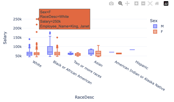
4. HW

아래의 코드를 활용하여 Kaggle의 HRdataset을 불러오고 물음에 답하라.

df = pd.read_csv('https://raw.githubusercontent.com/guebin/DV2022/master/posts/HRDataset_v14.csv')
df

	Employee_Name	EmpID	MarriedID	MaritalStatusID	GenderID	EmpStatusID	DeptID	PerfScoreID	FromDiversityJobFairID	Salary	...	ManagerName	ManagerID	RecruitmentSource	PerformanceScore	EngagementSurvey	EmpSatisfaction	SpecialProjectsCount	LastPerformanceReview_Date	DaysLateLast30	Absences
0	Adinolfi, Wilson K	10026	0	0	1	1	5	4	0	62506	...	Michael Albert	22.0	LinkedIn	Exceeds	4.60	5	0	1/17/2019	0	1
1	Ait Sidi, Karthikeyan	10084	1	1	1	5	3	3	0	104437	...	Simon Roup	4.0	Indeed	Fully Meets	4.96	3	6	2/24/2016	0	17
2	Akinkuolie, Sarah	10196	1	1	0	5	5	3	0	64955	...	Kissy Sullivan	20.0	LinkedIn	Fully Meets	3.02	3	0	5/15/2012	0	3
3	Alagbe,Trina	10088	1	1	0	1	5	3	0	64991	...	Elijiah Gray	16.0	Indeed	Fully Meets	4.84	5	0	1/3/2019	0	15
4	Anderson, Carol	10069	0	2	0	5	5	3	0	50825	...	Webster Butler	39.0	Google Search	Fully Meets	5.00	4	0	2/1/2016	0	2
...	...	...	...	...	...	...	...	...	...	...	...	...	...	...	...	...	...	...	...	...	...
306	Woodson, Jason	10135	0	0	1	1	5	3	0	65893	...	Kissy Sullivan	20.0	LinkedIn	Fully Meets	4.07	4	0	2/28/2019	0	13
307	Ybarra, Catherine	10301	0	0	0	5	5	1	0	48513	...	Brannon Miller	12.0	Google Search	PIP	3.20	2	0	9/2/2015	5	4
308	Zamora, Jennifer	10010	0	0	0	1	3	4	0	220450	...	Janet King	2.0	Employee Referral	Exceeds	4.60	5	6	2/21/2019	0	16
309	Zhou, Julia	10043	0	0	0	1	3	3	0	89292	...	Simon Roup	4.0	Employee Referral	Fully Meets	5.00	3	5	2/1/2019	0	11
310	Zima, Colleen	10271	0	4	0	1	5	3	0	45046	...	David Stanley	14.0	LinkedIn	Fully Meets	4.50	5	0	1/30/2019	0	2

311 rows × 36 columns

아래와 같은 시각화를 하라. (Employee_Name이 보이도록 할 것)

1. 강의영상

2. Imports

3. 여러가지 플랏

A. .plot.bar()

B. .plot.line()

C. .plot.scatter()

D. .plot.box()

E. .plot.hist()

F. .plot.area()