08wk-1: 에너지사용량 시각화

plotnine

Author

최규빈

Published

October 23, 2023

1. 강의영상

2. Imports

import pandas as pd 
import numpy as np
from plotnine import *

3. 예비학습

A. `pd.concat()`

# 예시1 – 위아래로

df1 = pd.DataFrame({'A':[1,2,3],'B':[2,3,4]})
df2 = pd.DataFrame({'A':[-1,-2,-3],'B':[-2,-3,-4]})

display("df1",df1)
display("df2",df2)

'df1'

	A	B
0	1	2
1	2	3
2	3	4

'df2'

	A	B
0	-1	-2
1	-2	-3
2	-3	-4

#pd.concat([df1,df2],axis=0) # (3,2) concat (3,2) -> (6,4) 
pd.concat([df1,df2])

	A	B
0	1	2
1	2	3
2	3	4
0	-1	-2
1	-2	-3
2	-3	-4

인덱스를 재정리하고 싶다면?

pd.concat([df1,df2]).reset_index(drop=True)

	A	B
0	1	2
1	2	3
2	3	4
3	-1	-2
4	-2	-3
5	-3	-4

#

# 예시2 – 좌우로

df1 = pd.DataFrame({'A':[1,2,3],'B':[2,3,4]})
df2 = pd.DataFrame({'C':[-1,-2,-3],'D':[-2,-3,-4]})

display("df1",df1)
display("df2",df2)

'df1'

	A	B
0	1	2
1	2	3
2	3	4

'df2'

	C	D
0	-1	-2
1	-2	-3
2	-3	-4

pd.concat([df1,df2],axis=1) # (3,2) concat (3,2) -> (3,4)

	A	B	C	D
0	1	2	-1	-2
1	2	3	-2	-3
2	3	4	-3	-4

#

B. `pd.merge()`

big = pd.DataFrame({'department':['A','A','B','B'], 'gender':['male','female','male','female'],'count':[1,2,3,1]})
small = pd.DataFrame({'department':['A','B'], 'total':[3,4]})

display("big",big)
display("small",small)

'big'

	department	gender	count
0	A	male	1
1	A	female	2
2	B	male	3
3	B	female	1

'small'

	department	total
0	A	3
1	B	4

big.merge(small)

	department	gender	count	total
0	A	male	1	3
1	A	female	2	3
2	B	male	3	4
3	B	female	1	4

small.merge(big)

	department	total	gender	count
0	A	3	male	1
1	A	3	female	2
2	B	4	male	3
3	B	4	female	1

C. `.applymap()`

# 예시1

np.random.seed(43052)
df = pd.DataFrame({'A':np.random.rand(3), 'B':np.random.rand(3)})
df

	A	B
0	0.817682	0.619777
1	0.049532	0.122541
2	0.838686	0.117128

df.applymap(lambda x: 'Yes' if x>0.5 else 'No')

/tmp/ipykernel_288950/1665022133.py:1: FutureWarning: DataFrame.applymap has been deprecated. Use DataFrame.map instead.

	A	B
0	Yes	Yes
1	No	No
2	Yes	No

#

D. `df.astype()`

- 예시1

df = pd.DataFrame({'A':[0,1,2],'B':[4,5,6]})
df

	A	B
0	0	4
1	1	5
2	2	6

df.astype(float)

	A	B
0	0.0	4.0
1	1.0	5.0
2	2.0	6.0

E. 제 아픈기억

# 예제1 – object형은 일괄적으로 문자형임을 의미하는게 아님

np.random.seed(43052)
df = pd.DataFrame({'A':['1','2','0','1',2], 'B':['2','3','0','0',0]})
df

	A	B
0	1	2
1	2	3
2	0	0
3	1	0
4	2	0

df.info()

<class 'pandas.core.frame.DataFrame'>
RangeIndex: 5 entries, 0 to 4
Data columns (total 2 columns):
 #   Column  Non-Null Count  Dtype 
---  ------  --------------  ----- 
 0   A       5 non-null      object
 1   B       5 non-null      object
dtypes: object(2)
memory usage: 208.0+ bytes

df.A[0],df.A[4],df.B[0],df.B[4]

('1', 2, '2', 0)

#

# 예제2 – column이름이 이상하게 들어가 있는 경우가 있음.

df = pd.DataFrame({('A',''):[0,0,0], ('B',''):[1,1,1]})
df

	A	B

0	0	1
1	0	1
2	0	1

df['A']

0    0
1    0
2    0
Name: A, dtype: int64

df[('A','')]

0    0
1    0
2    0
Name: (A, ), dtype: int64

#

4. 에너지사용량 시각화

(1) 아래는 2019년 서울의 에너지사용량을 불러오는 예시코드이다.

pd.read_csv('https://raw.githubusercontent.com/guebin/DV2022/main/posts/Energy/Seoul2019.csv')

	지역	건물동수	연면적	에너지사용량(TOE)/전기	에너지사용량(TOE)/도시가스	에너지사용량(TOE)/지역난방
0	종로구	17,851	9,204,140	63,492	76,653	799
1	중구	10,383	10,078,848	79,223	68,210	497
2	용산구	17,138	10,756,612	51,229	79,805	11,128
3	성동구	13,980	11,804,313	59,832	99,986	0
4	광진구	21,556	12,272,738	68,756	123,447	0
5	동대문구	21,794	12,664,554	65,913	111,420	0
6	중랑구	23,950	15,182,802	59,370	109,284	7,442
7	성북구	27,112	15,938,807	77,007	148,376	0
8	강북구	23,334	9,458,987	47,731	100,045	0
9	도봉구	13,168	10,644,704	44,985	90,379	5,268
10	노원구	9,704	17,197,086	77,010	94,340	50,859
11	은평구	25,200	14,735,131	75,914	130,159	14,370
12	서대문구	17,651	12,559,425	65,164	111,542	6,330
13	마포구	18,844	15,024,186	92,453	114,931	20,148
14	양천구	14,690	15,428,339	70,721	82,857	49,258
15	강서구	20,446	20,641,866	86,809	128,786	35,896
16	구로구	17,204	13,509,894	59,916	120,457	2,963
17	금천구	12,135	7,420,441	34,791	69,814	732
18	영등포구	18,133	14,914,027	87,480	114,238	13,531
19	동작구	20,102	13,612,946	66,811	132,285	899
20	관악구	26,460	14,997,859	85,416	158,543	0
21	서초구	12,856	21,560,285	135,491	121,437	38,866
22	강남구	16,129	29,961,585	180,121	149,045	83,459
23	송파구	19,331	26,573,343	139,117	143,601	71,954
24	강동구	16,636	15,048,315	70,341	121,931	11,921

에너지 사용량은 2018년부터 2021년까지의 기간 동안 서울, 부산 등 여러 지역에 대해 정리되어 있으며, 아래 주소 형식으로 저장되어 있다.

https://raw.githubusercontent.com/guebin/DV2022/main/posts/Energy/Seoul2018.csv
https://raw.githubusercontent.com/guebin/DV2022/main/posts/Energy/Seoul2019.csv
https://raw.githubusercontent.com/guebin/DV2022/main/posts/Energy/Seoul2020.csv
https://raw.githubusercontent.com/guebin/DV2022/main/posts/Energy/Seoul2021.csv
...
https://raw.githubusercontent.com/guebin/DV2022/main/posts/Energy/Busan2018.csv
https://raw.githubusercontent.com/guebin/DV2022/main/posts/Energy/Busan2019.csv
https://raw.githubusercontent.com/guebin/DV2022/main/posts/Energy/Busan2020.csv
https://raw.githubusercontent.com/guebin/DV2022/main/posts/Energy/Busan2021.csv

아래의 url, prov를 참고하여 모든 자료를 불러온 뒤 pd.concat()을 이용하여 하나의 df로 합쳐라.

url = 'https://raw.githubusercontent.com/guebin/DV2022/main/posts/Energy/{}.csv'

prov = ['Seoul', 'Busan', 'Daegu', 'Incheon', 
        'Gwangju', 'Daejeon', 'Ulsan', 'Sejongsi', 
        'Gyeonggi-do', 'Gangwon-do', 'Chungcheongbuk-do', 
        'Chungcheongnam-do', 'Jeollabuk-do', 'Jeollanam-do', 
        'Gyeongsangbuk-do', 'Gyeongsangnam-do', 'Jeju-do']

올바르게 정리된 데이터프레임의 예시는 아래와 같다.

(풀이)

df = pd.concat([pd.read_csv(url.format(p+y)).assign(년도=y, 시도=p) for p in prov for y in ['2018', '2019', '2020', '2021']]).reset_index(drop=True)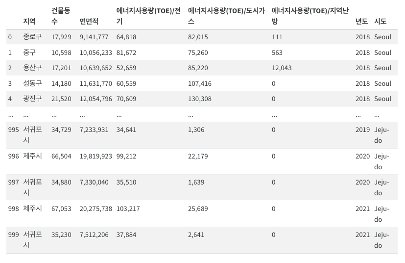
df

	지역	건물동수	연면적	에너지사용량(TOE)/전기	에너지사용량(TOE)/도시가스	에너지사용량(TOE)/지역난방	년도	시도
0	종로구	17,929	9,141,777	64,818	82,015	111	2018	Seoul
1	중구	10,598	10,056,233	81,672	75,260	563	2018	Seoul
2	용산구	17,201	10,639,652	52,659	85,220	12,043	2018	Seoul
3	성동구	14,180	11,631,770	60,559	107,416	0	2018	Seoul
4	광진구	21,520	12,054,796	70,609	130,308	0	2018	Seoul
...	...	...	...	...	...	...	...	...
995	서귀포시	34,729	7,233,931	34,641	1,306	0	2019	Jeju-do
996	제주시	66,504	19,819,923	99,212	22,179	0	2020	Jeju-do
997	서귀포시	34,880	7,330,040	35,510	1,639	0	2020	Jeju-do
998	제주시	67,053	20,275,738	103,217	25,689	0	2021	Jeju-do
999	서귀포시	35,230	7,512,206	37,884	2,641	0	2021	Jeju-do

1000 rows × 8 columns

(2) 의미상 숫자형이지만 문자형으로 입력이된 자료를 모두 전처리하라.

(풀이)

df.assign(년도 = df.년도.astype(int))\
.set_index(['년도','시도','지역']).applymap(lambda x: int(str(x).replace(',','')))\
.reset_index()

/tmp/ipykernel_322791/847505444.py:2: FutureWarning: DataFrame.applymap has been deprecated. Use DataFrame.map instead.

	년도	시도	지역	건물동수	연면적	에너지사용량(TOE)/전기	에너지사용량(TOE)/도시가스	에너지사용량(TOE)/지역난방
0	2018	Seoul	종로구	17929	9141777	64818	82015	111
1	2018	Seoul	중구	10598	10056233	81672	75260	563
2	2018	Seoul	용산구	17201	10639652	52659	85220	12043
3	2018	Seoul	성동구	14180	11631770	60559	107416	0
4	2018	Seoul	광진구	21520	12054796	70609	130308	0
...	...	...	...	...	...	...	...	...
995	2019	Jeju-do	서귀포시	34729	7233931	34641	1306	0
996	2020	Jeju-do	제주시	66504	19819923	99212	22179	0
997	2020	Jeju-do	서귀포시	34880	7330040	35510	1639	0
998	2021	Jeju-do	제주시	67053	20275738	103217	25689	0
999	2021	Jeju-do	서귀포시	35230	7512206	37884	2641	0

1000 rows × 8 columns

(3) 열의 이름을 아래와 같이 바꾸라.

name_dict = {
    '년도': 'Year',
    '시도': 'Prov',
    '지역': 'Reg',
    '건물동수': 'BldgCount',
    '연면적': 'Area',
    '에너지사용량(TOE)/전기': 'Elec',
    '에너지사용량(TOE)/도시가스': 'Gas',
    '에너지사용량(TOE)/지역난방': 'Heat'
}

(풀이)

df.assign(년도 = df.년도.astype(int))\
.set_index(['년도','시도','지역']).applymap(lambda x: int(str(x).replace(',','')))\
.reset_index().rename(name_dict,axis=1)

/tmp/ipykernel_322791/1695199233.py:2: FutureWarning: DataFrame.applymap has been deprecated. Use DataFrame.map instead.

	Year	Prov	Reg	BldgCount	Area	Elec	Gas	Heat
0	2018	Seoul	종로구	17929	9141777	64818	82015	111
1	2018	Seoul	중구	10598	10056233	81672	75260	563
2	2018	Seoul	용산구	17201	10639652	52659	85220	12043
3	2018	Seoul	성동구	14180	11631770	60559	107416	0
4	2018	Seoul	광진구	21520	12054796	70609	130308	0
...	...	...	...	...	...	...	...	...
995	2019	Jeju-do	서귀포시	34729	7233931	34641	1306	0
996	2020	Jeju-do	제주시	66504	19819923	99212	22179	0
997	2020	Jeju-do	서귀포시	34880	7330040	35510	1639	0
998	2021	Jeju-do	제주시	67053	20275738	103217	25689	0
999	2021	Jeju-do	서귀포시	35230	7512206	37884	2641	0

1000 rows × 8 columns

(4) 아래와 같은 그림을 시각화 하라.

# 시각화예시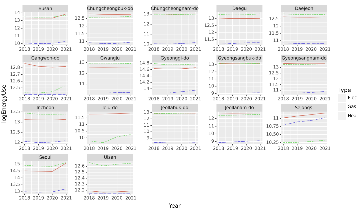

(풀이)

tidydata = df.assign(년도 = df.년도.astype(int))\
.set_index(['년도','시도','지역']).applymap(lambda x: int(str(x).replace(',','')))\
.reset_index().rename(name_dict,axis=1)\
.drop(['BldgCount','Area'],axis=1)\
.set_index(['Year','Prov','Reg']).stack().reset_index()\
.rename({'level_3':'Type',0:'EnergyUse'},axis=1)\
.pivot_table(index=['Year','Prov','Type'],values='EnergyUse',aggfunc='sum')\
.reset_index()\
.eval('logEnergyUse = log(EnergyUse)')
tidydata 
# --- # 
fig = ggplot(tidydata) 
line = geom_line(aes(x='Year',y='logEnergyUse',color='Type',linetype='Type'))
fig = (fig + line + facet_wrap('Prov',scales='free')).draw()
fig

/tmp/ipykernel_322791/2236388880.py:2: FutureWarning: DataFrame.applymap has been deprecated. Use DataFrame.map instead.
/home/cgb2/anaconda3/envs/ag/lib/python3.10/site-packages/pandas/core/arraylike.py:396: RuntimeWarning: divide by zero encountered in log

fig.set_size_inches(10,6)
fig.set_dpi(150)
fig

(5) Prov별로 총 에너지사용량이 많은 상위5개의 Reg을 찾고 아래와 같이 시각화 하라.

# 시각화예시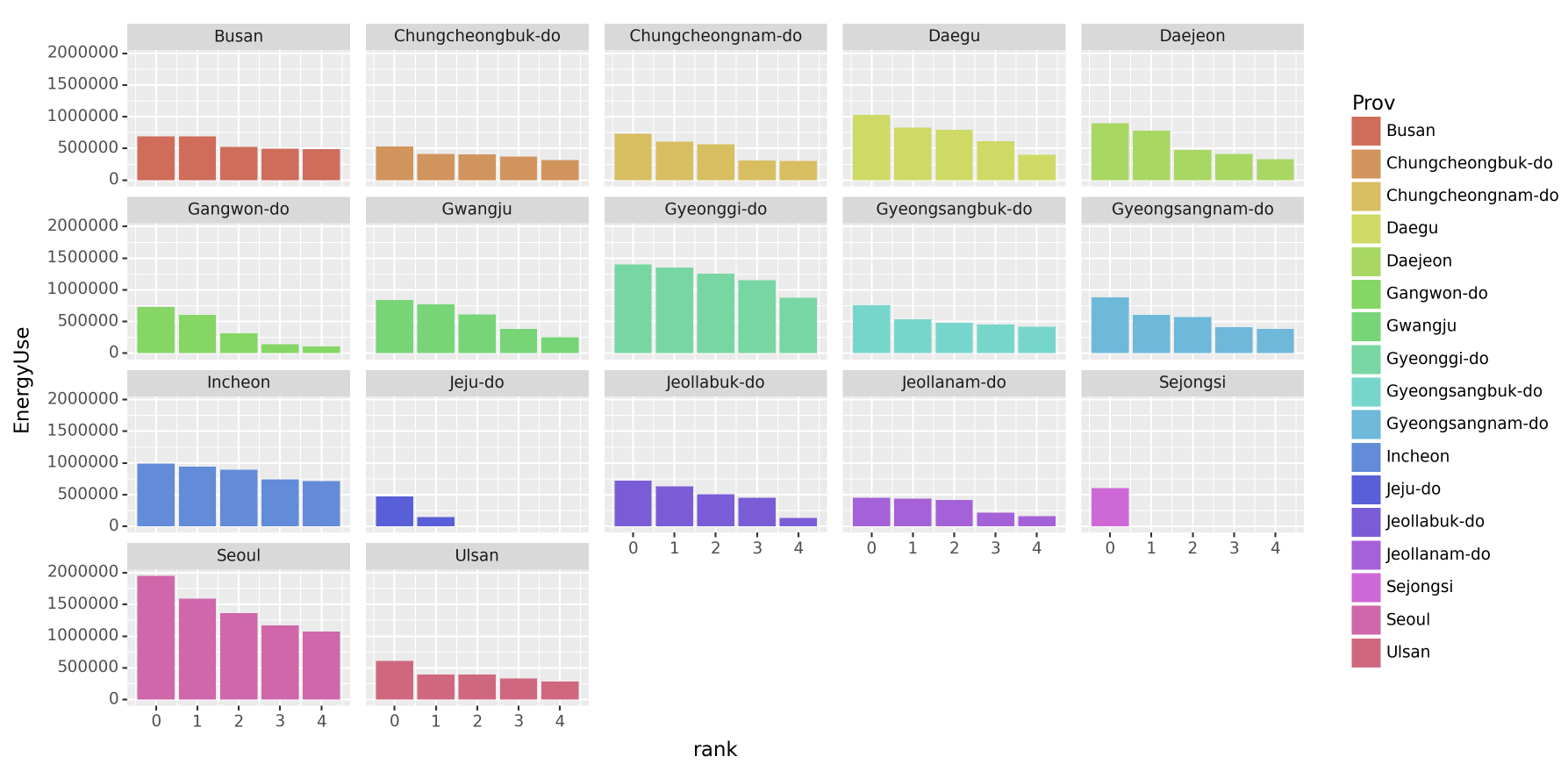

(풀이)

df.assign(년도 = df.년도.astype(int))\
.set_index(['년도','시도','지역']).applymap(lambda x: int(str(x).replace(',','')))\
.reset_index().rename(name_dict,axis=1)\
.eval('EnergyUse = Elec + Gas + Heat')\
.drop(['BldgCount','Area','Elec','Gas','Heat'],axis=1)\
.pivot_table(index=['Prov','Reg'],columns='Year',values='EnergyUse').sum(axis=1)\
.reset_index().rename({0:'EnergyUse'},axis=1)

/tmp/ipykernel_322791/1149148944.py:2: FutureWarning: DataFrame.applymap has been deprecated. Use DataFrame.map instead.

	Prov	Reg	EnergyUse
0	Busan	강서구	200386.0
1	Busan	금정구	451212.0
2	Busan	기장군	287926.0
3	Busan	남구	491030.0
4	Busan	동구	156302.0
...	...	...	...
245	Ulsan	남구	607820.0
246	Ulsan	동구	281094.0
247	Ulsan	북구	334844.0
248	Ulsan	울주군	394217.0
249	Ulsan	중구	395158.0

250 rows × 3 columns

g = df.assign(년도 = df.년도.astype(int))\
.set_index(['년도','시도','지역']).applymap(lambda x: int(str(x).replace(',','')))\
.reset_index().rename(name_dict,axis=1)\
.eval('EnergyUse = Elec + Gas + Heat')\
.drop(['BldgCount','Area','Elec','Gas','Heat'],axis=1)\
.pivot_table(index=['Prov','Reg'],columns='Year',values='EnergyUse').sum(axis=1)\
.reset_index().rename({0:'EnergyUse'},axis=1)\
.groupby('Prov')

/tmp/ipykernel_322791/1748878604.py:2: FutureWarning: DataFrame.applymap has been deprecated. Use DataFrame.map instead.

tidydata = pd.concat([df.sort_values('EnergyUse',ascending=False).reset_index(drop=True).reset_index().rename({'index':'Rank'},axis=1).iloc[:5] for k,df in g])\
.reset_index(drop=True)
tidydata 
#---# 
fig = (ggplot(tidydata) + geom_col(aes(x='Rank',y='EnergyUse',fill='Prov')) + facet_wrap('Prov')).draw()
fig.set_size_inches(10,5)
fig.set_dpi(150)
fig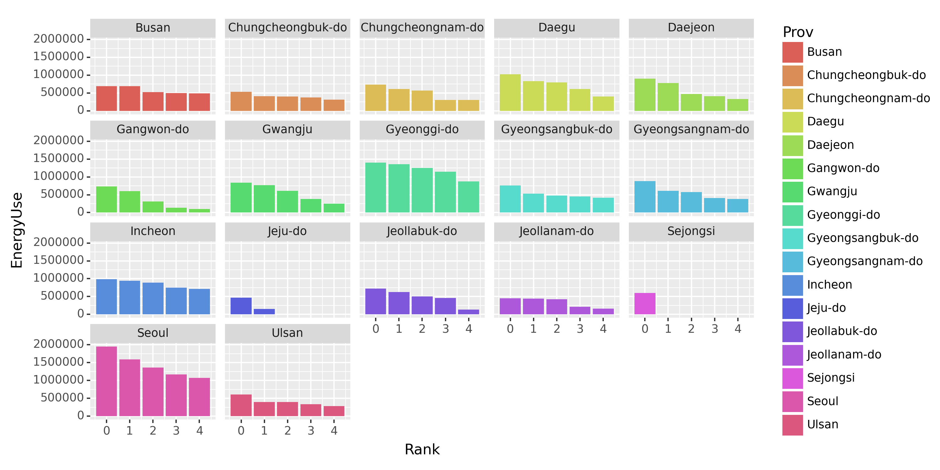

(5) (Prov,Year)별 전기에너지 사용량 비율을 구하고 아래와 같이 시각화 하라. + 제주를 제외한 지역으로 한정하고 시각화하라.

# 시각화예시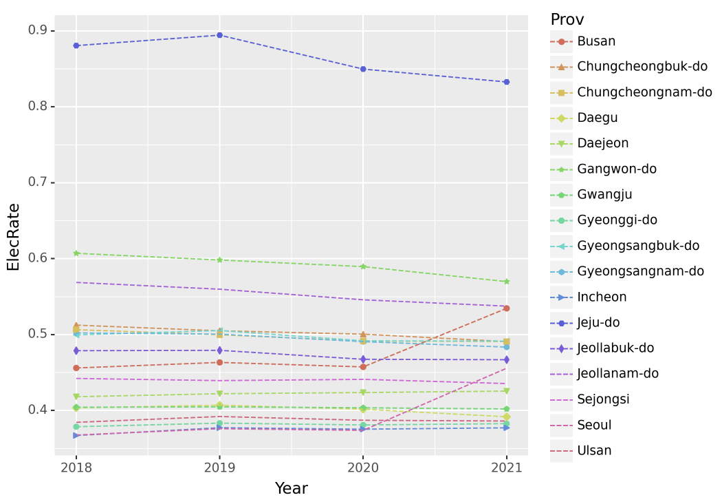

(풀이1) – 수업시간에 한 풀이

df.assign(년도 = df.년도.astype(int))\
.set_index(['년도','시도','지역']).applymap(lambda x: int(str(x).replace(',','')))\
.reset_index().rename(name_dict,axis=1)\
.drop(['BldgCount','Area'],axis=1).melt(id_vars=['Year','Prov','Reg'])\
.rename({'variable':'Type','value':'EnergyUse'},axis=1)\
.pivot_table(index=['Prov','Year'],columns='Type',values='EnergyUse',aggfunc='sum')\
.eval('ElecRate = Elec/(Elec+Gas+Heat)').loc[:,'ElecRate'].reset_index()

/tmp/ipykernel_322791/3362619229.py:2: FutureWarning: DataFrame.applymap has been deprecated. Use DataFrame.map instead.

	Prov	Year	ElecRate
0	Busan	2018	0.455996
1	Busan	2019	0.463324
2	Busan	2020	0.457401
3	Busan	2021	0.534566
4	Chungcheongbuk-do	2018	0.512447
...	...	...	...
63	Seoul	2021	0.455675
64	Ulsan	2018	0.384385
65	Ulsan	2019	0.392067
66	Ulsan	2020	0.387118
67	Ulsan	2021	0.386115

68 rows × 3 columns

tidydata = df.assign(년도 = df.년도.astype(int))\
.set_index(['년도','시도','지역']).applymap(lambda x: int(str(x).replace(',','')))\
.reset_index().rename(name_dict,axis=1)\
.drop(['BldgCount','Area'],axis=1).melt(id_vars=['Year','Prov','Reg'])\
.rename({'variable':'Type','value':'EnergyUse'},axis=1)\
.pivot_table(index=['Prov','Year'],columns='Type',values='EnergyUse',aggfunc='sum')\
.eval('ElecRate = Elec/(Elec+Gas+Heat)').loc[:,'ElecRate'].reset_index()
#--#
fig = ggplot(tidydata)
point = geom_point(aes(x='Year',y='ElecRate',color='Prov',shape='Prov'))
line = geom_line(aes(x='Year',y='ElecRate',color='Prov'),linetype='dashed')
fig = (fig + point + line).draw()
fig.set_dpi(150)
fig

/tmp/ipykernel_322791/3057913787.py:2: FutureWarning: DataFrame.applymap has been deprecated. Use DataFrame.map instead.
/home/cgb2/anaconda3/envs/ag/lib/python3.10/site-packages/mizani/palettes.py:706: UserWarning: Palette can return a maximum of 13 values. 17 values requested.
/home/cgb2/anaconda3/envs/ag/lib/python3.10/site-packages/plotnine/layer.py:364: PlotnineWarning: geom_point : Removed 16 rows containing missing values.
/home/cgb2/anaconda3/envs/ag/lib/python3.10/site-packages/mizani/palettes.py:706: UserWarning: Palette can return a maximum of 13 values. 17 values requested.
/home/cgb2/anaconda3/envs/ag/lib/python3.10/site-packages/plotnine/guides/guides.py:259: PlotnineWarning: geom_point legend : Removed 4 rows containing missing values.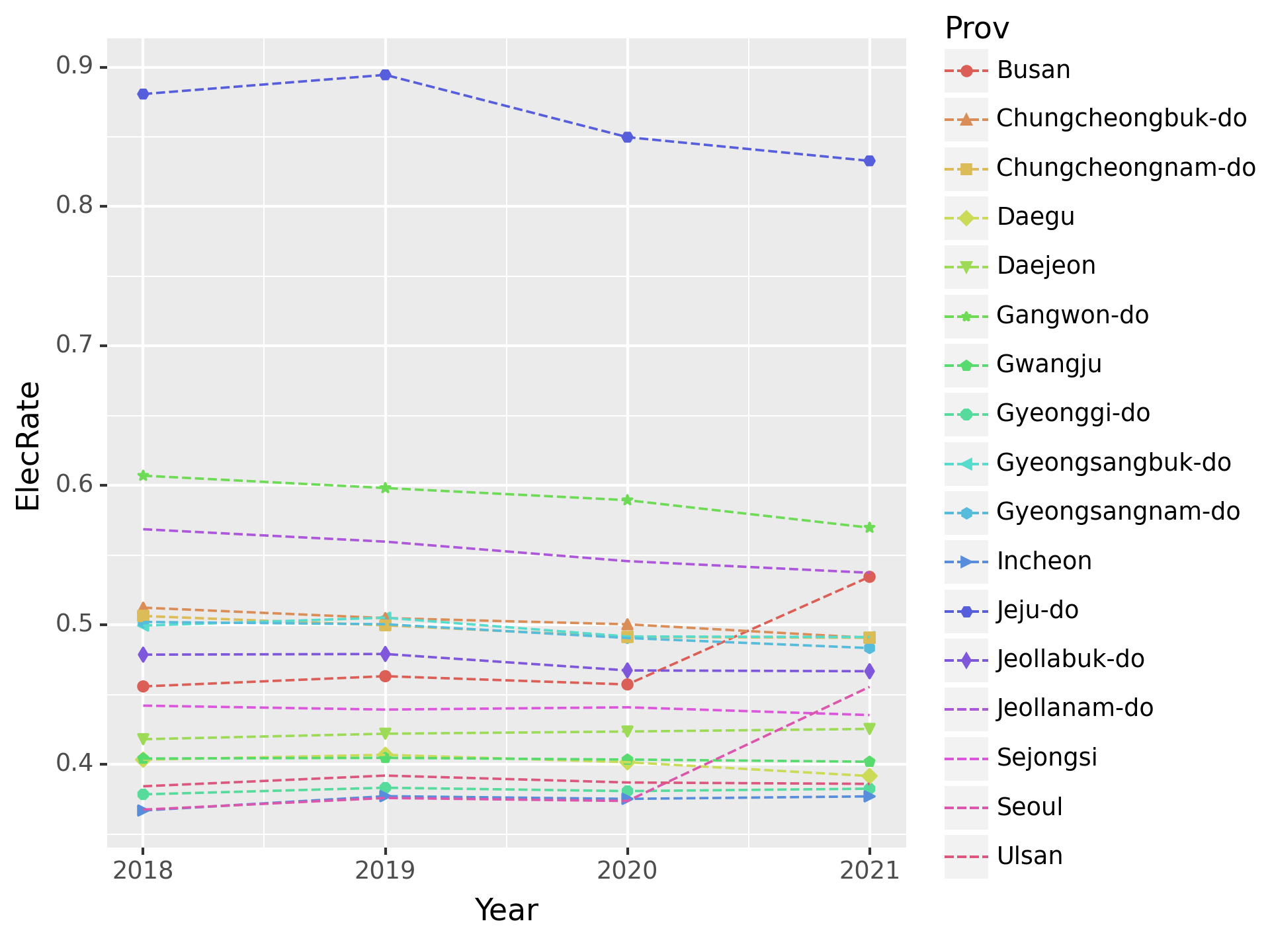

fig = ggplot(tidydata.query("Prov != 'Jeju-do'"))
point = geom_point(aes(x='Year',y='ElecRate',color='Prov',shape='Prov'))
line = geom_line(aes(x='Year',y='ElecRate',color='Prov'),linetype='dashed')
fig = (fig + point + line).draw()
fig.set_dpi(150)
fig

/home/cgb2/anaconda3/envs/ag/lib/python3.10/site-packages/mizani/palettes.py:706: UserWarning: Palette can return a maximum of 13 values. 16 values requested.
/home/cgb2/anaconda3/envs/ag/lib/python3.10/site-packages/plotnine/layer.py:364: PlotnineWarning: geom_point : Removed 12 rows containing missing values.
/home/cgb2/anaconda3/envs/ag/lib/python3.10/site-packages/mizani/palettes.py:706: UserWarning: Palette can return a maximum of 13 values. 16 values requested.
/home/cgb2/anaconda3/envs/ag/lib/python3.10/site-packages/plotnine/guides/guides.py:259: PlotnineWarning: geom_point legend : Removed 3 rows containing missing values.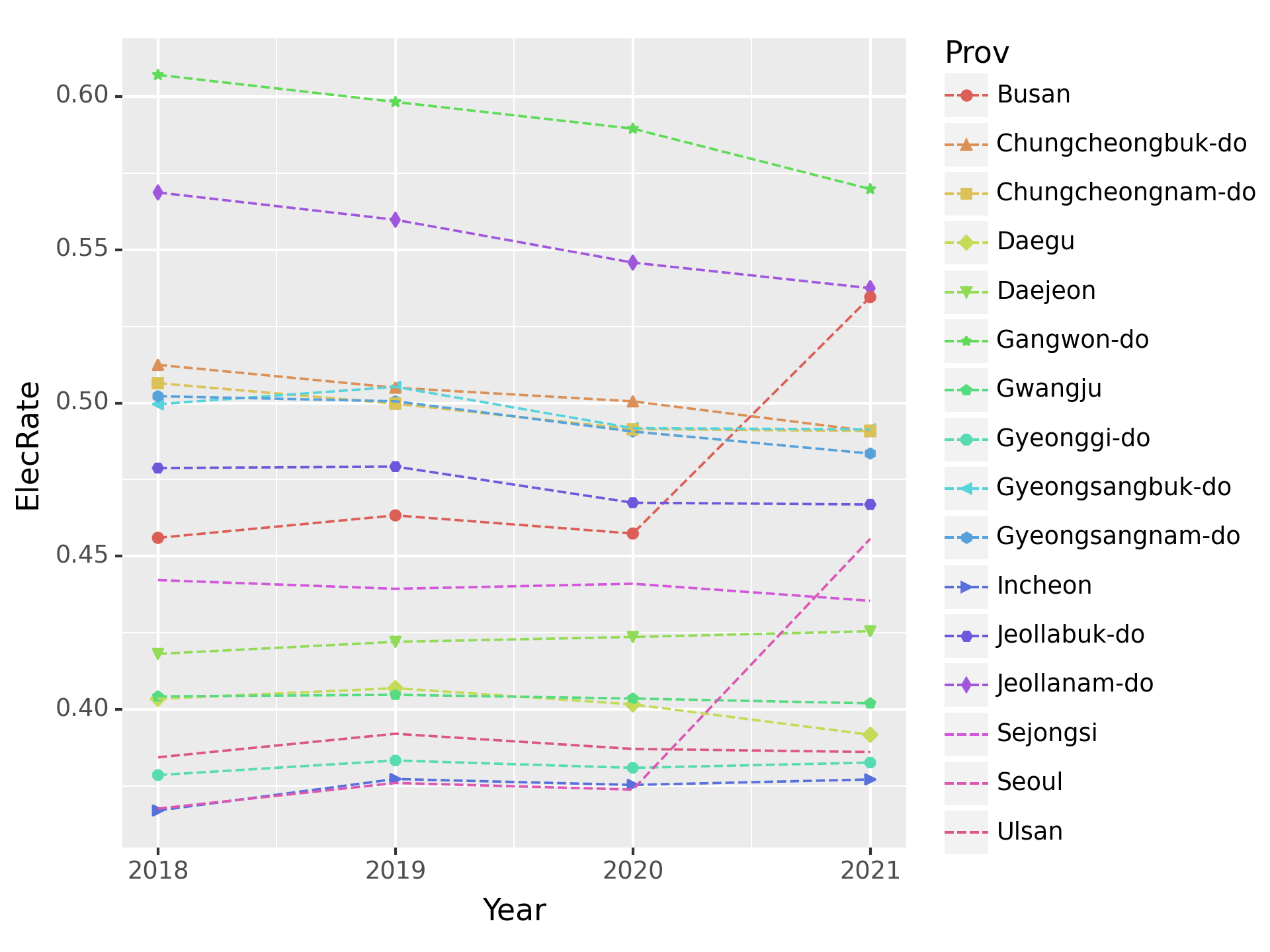

(풀이2) – draft에 있던 풀이, 수업시간에 풀이한것과 약간다름

df.assign(년도 = df.년도.astype(int))\
    .set_index(['년도','시도','지역']).applymap(lambda x: str(x).replace(',','')).astype(int).reset_index()\
    .rename(name_dict,axis=1)\
    .drop(['BldgCount','Area'],axis=1)\
    .melt(id_vars=['Year','Prov','Reg']).rename({'variable':'Type','value':'EnergyUse'},axis=1)\
    .pivot_table(index=['Year','Prov','Type'],values='EnergyUse',aggfunc='sum').reset_index()\
    .set_index(['Year','Prov','Type']).unstack()\
    .assign(ElecRate = lambda df: df[('EnergyUse','Elec')]/(df[('EnergyUse','Elec')]+df[('EnergyUse','Gas')]+df[('EnergyUse','Heat')]))\
    .iloc[:,-1].reset_index().set_axis(['Year','Prov','ElecRate'],axis=1)

/tmp/ipykernel_322791/2924150206.py:2: FutureWarning: DataFrame.applymap has been deprecated. Use DataFrame.map instead.

	Year	Prov	ElecRate
0	2018	Busan	0.455996
1	2018	Chungcheongbuk-do	0.512447
2	2018	Chungcheongnam-do	0.506471
3	2018	Daegu	0.403464
4	2018	Daejeon	0.418136
...	...	...	...
63	2021	Jeollabuk-do	0.466878
64	2021	Jeollanam-do	0.537464
65	2021	Sejongsi	0.435457
66	2021	Seoul	0.455675
67	2021	Ulsan	0.386115

68 rows × 3 columns

이후의 과정은 풀이1와 같음.

5. `pd.merge()` 의 이용

before에서 after로 가는 일반적인 방법이 있을까?

before = df.assign(년도 = df.년도.astype(int))\
    .set_index(['년도','시도','지역']).applymap(lambda x: str(x).replace(',','')).astype(int).reset_index()\
    .rename(name_dict,axis=1)\
    .drop(['BldgCount','Area'],axis=1)
after = before\
    .melt(id_vars=['Year','Prov','Reg']).rename({'variable':'Type','value':'EnergyUse'},axis=1)\
    .pivot_table(index=['Year','Prov','Type'],values='EnergyUse',aggfunc='sum').reset_index()\
    .set_index(['Year','Prov','Type']).unstack()\
    .assign(ElecRate = lambda df: df[('EnergyUse','Elec')]/(df[('EnergyUse','Elec')]+df[('EnergyUse','Gas')]+df[('EnergyUse','Heat')]))\
    .iloc[:,-1].reset_index().set_axis(['Year','Prov','ElecRate'],axis=1)
display('before',before)
display('after',after)

/tmp/ipykernel_322791/2643872.py:2: FutureWarning: DataFrame.applymap has been deprecated. Use DataFrame.map instead.

'before'

	Year	Prov	Reg	Elec	Gas	Heat
0	2018	Seoul	종로구	64818	82015	111
1	2018	Seoul	중구	81672	75260	563
2	2018	Seoul	용산구	52659	85220	12043
3	2018	Seoul	성동구	60559	107416	0
4	2018	Seoul	광진구	70609	130308	0
...	...	...	...	...	...	...
995	2019	Jeju-do	서귀포시	34641	1306	0
996	2020	Jeju-do	제주시	99212	22179	0
997	2020	Jeju-do	서귀포시	35510	1639	0
998	2021	Jeju-do	제주시	103217	25689	0
999	2021	Jeju-do	서귀포시	37884	2641	0

1000 rows × 6 columns

'after'

	Year	Prov	ElecRate
0	2018	Busan	0.455996
1	2018	Chungcheongbuk-do	0.512447
2	2018	Chungcheongnam-do	0.506471
3	2018	Daegu	0.403464
4	2018	Daejeon	0.418136
...	...	...	...
63	2021	Jeollabuk-do	0.466878
64	2021	Jeollanam-do	0.537464
65	2021	Sejongsi	0.435457
66	2021	Seoul	0.455675
67	2021	Ulsan	0.386115

68 rows × 3 columns

(해법) – 머리가 안돌아가면 일단 tidydata로 만들고 시작..

small = before.melt(id_vars=['Year','Prov','Reg'])\
.groupby(['Year','Prov']).agg({'value':'sum'}).reset_index()\
.rename({'value':'EnergyUseTotal'},axis=1)

big = before.melt(id_vars=['Year','Prov','Reg'])\
.groupby(['Year','Prov','variable']).agg({'value':'sum'}).reset_index()\
.rename({'variable':'Type','value':'EnergyUse'},axis=1)

big.merge(small).query('Type=="Elec"')\
.eval('ElecRate = EnergyUse/EnergyUseTotal')\
.loc[:,['Year','Prov','ElecRate']].reset_index(drop=True)

	Year	Prov	ElecRate
0	2018	Busan	0.455996
1	2018	Chungcheongbuk-do	0.512447
2	2018	Chungcheongnam-do	0.506471
3	2018	Daegu	0.403464
4	2018	Daejeon	0.418136
...	...	...	...
63	2021	Jeollabuk-do	0.466878
64	2021	Jeollanam-do	0.537464
65	2021	Sejongsi	0.435457
66	2021	Seoul	0.455675
67	2021	Ulsan	0.386115

68 rows × 3 columns

1. 강의영상

2. Imports

3. 예비학습

A. pd.concat()

B. pd.merge()

C. .applymap()

D. df.astype()

E. 제 아픈기억

4. 에너지사용량 시각화

5. pd.merge() 의 이용

6. HW 없음

A. `pd.concat()`

B. `pd.merge()`

C. `.applymap()`

D. `df.astype()`

5. `pd.merge()` 의 이용