DV2022 - midterm

중간고사

import numpy as np
import matplotlib.pyplot as plt 
import pandas as pd
import seaborn as sns
from plotnine import *

`1`. 시각화의 해석 - 다음을 잘 읽고 물음에 답하라. (20점)

(1) 아래의 그림을 보고 올바르게 해석한 것을 고르라. (모두 맞출경우만 정답으로 인정)

#hide_input
x = [10, 8, 13, 9, 11, 14, 6, 4, 12, 7, 5]
y1 = [8.04, 6.95, 7.58, 8.81, 8.33, 9.96, 7.24, 4.26, 10.84, 4.82, 5.68]
y2 = [9.14, 8.14, 8.74, 8.77, 9.26, 8.10, 6.13, 3.10, 9.13, 7.26, 4.74]
y3 = [7.46, 6.77, 12.74, 7.11, 7.81, 8.84, 6.08, 5.39, 8.15, 6.42, 5.73]
x4 = [8, 8, 8, 8, 8, 8, 8, 19, 8, 8, 8]
y4 = [6.58, 5.76, 7.71, 8.84, 8.47, 7.04, 5.25, 12.50, 5.56, 7.91, 6.89]
fig, ((ax1,ax2),(ax3,ax4)) = plt.subplots(2,2)
ax1.plot(x,y1,'.') 
ax1.set_title("(a)")
ax2.plot(x,y2,'.') 
ax2.set_title("(b)")
ax3.plot(x,y3,'.'); ax3.plot(x[2],y3[2],'o',color='C1') 
ax3.set_title("(c)")
ax4.plot(x4,y4,'.'); ax4.plot(x4[-4],y4[-4],'o',color='C1')
ax4.set_title("(d)")
fig.suptitle("Anscombe's quartet",size=15)
plt.tight_layout()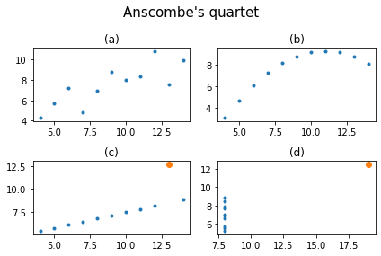

소윤: (a)의 경우 \((x_i,y_i)\)의 산점도가 직선형태이므로 표본상관계수의 값을 해석하는 것이 두 자료의 관계를 파악할때 도움을 준다.
다호: (b)의 경우 \((x_i,y_i)\)의 산점도가 이차곡선이므로 표본상관계수의 해석으로 두 자료의 관계를 모두 파악할 수 없다.
하니: (c)의 경우 주황색으로 표시된 점을 제외한다면 표본상관계수로 자료를 해석하기에 바람직하다.
도한: (d)도 (c)와 마찬가지로 주황색으로 표시된 점을 제외한다면 표본상관계수로 자료를 해석하기에 바람직하다.

(풀이)

정답: 소윤, 다호, 하니가 맞게 서술함.
도한이 틀린이유: 주황색점을 제외할 경우 \(x\)의 변화량이 0이므로 분모가 0으로 수렴. 따라서 상관계수의 해석이 무의미하다.

(2) 아래의 그림을 보고 올바르게 해석한 것을 모두 고르라. (모두 맞출경우만 정답으로 인정) - 그림에 대한 배경설명은 10월17일,19일의 “아이스크림을 많이 먹으면 걸리는 병”을 참고

#hide_input
df=pd.read_csv('https://raw.githubusercontent.com/guebin/DV2022/master/_notebooks/icecream.csv')
ggplot(data=df.assign(temp=pd.cut(df.temp,[-np.inf,0,5,10,15,20,25,30,np.inf])))\
+geom_point(aes(x='icecream',y='disease',color='temp'))\
+geom_smooth(aes(x='icecream',y='disease',color='temp'))

/home/cgb4/anaconda3/envs/py37/lib/python3.7/site-packages/plotnine/stats/smoothers.py:311: PlotnineWarning: Confidence intervals are not yet implementedfor lowess smoothings.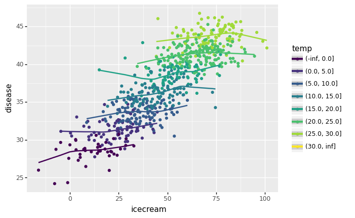

<ggplot: (8776319243321)>

소윤: 아이스크림과 소아마비는 상관계수는 양수이다.
다호: 상관계수가 양수라는 정보만으로는 소아마비와 아이스크림사이에 인과성이 있다고 주장하기 어렵다.
하니: 소아마비와 아이스크림 사이에 존재하는 은닉변수 온도를 통제한다면 소아마비와 아이스크림 사이의 상관계수는 0에 가깝다.
도한: 하니의 분석에 따르면 소아마비와 아이스크림 사이의 인과성은 없다고 보아야 한다. (단 소아마비와 아이스크림 사이의 은닉된 변수는 온도가 유일하다고 가정한다)

(풀이)

정답: 소윤, 다호, 하니, 도한 모두 맞게 서술함

`2`. 시각화구현 I - 다음을 잘 읽고 물음에 답하라. (10점)

(1)~(3) 주어진 자료에 대하여 다음을 시각화 하라. (maplotlib 이용)

x=[1,2,3,4]
y=[1,2,3,2]

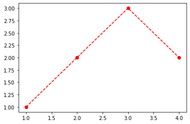
(1) 출제의도: 마커변경, 색깔변경

plt.plot(x,y,'x',color='C1');

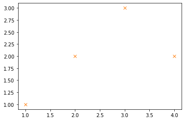
채점기준: 색깔이 정확하게 일치하지 않을 경우 0점으로 처리

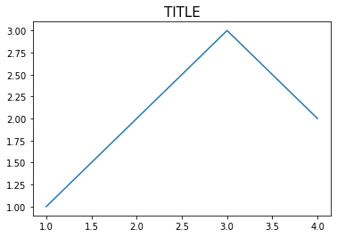
(2) 출제의도: title설정

plt.plot(x,y,)
plt.title('TITLE',size=15);

(3) 출제의도: linetype 변경, dot connected-plot

plt.plot(x,y,'or--');

(4) ~ (5) 주어진 자료에 대하여 다음을 시각화 하라.

x=[1,2,3,4]
y1=[1,2,4,3]
y2=[1.1,1.9,3,5]

(4) 출제의도: legend

plt.plot(x,y1,'o--',label='y1')
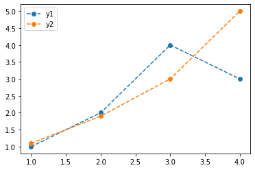
plt.plot(x,y2,'o--',label='y2')
plt.legend();

(5) 출제의도: linetype, linewidth 변경

fig,ax = plt.subplots(1,2)
ax[0].plot(x,y1,'--',lw=2)
ax[1].plot(x,y2,'--',lw=4);

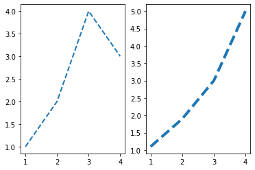
채점기준: 선의두께가 예시와 조금 달라도 만점으로 인정 (두께의 변화만 있으면 정답으로 인정함)

`3`. 시각화구현 II – 다음을 잘 읽고 물음에 답하라. (10점)

주어진 자료가 아래와 같다고 하자.

np.random.seed(43052)
x1,y1 =  np.random.multivariate_normal([-2,-2],[[1,-0.8],[-0.8,1]],size=500).T
x2,y2 =  np.random.multivariate_normal([2,2],[[1,-0.7],[-0.7,1]],size=500).T

(1) matplotlib와 seaborn을 이용하여 아래와 같이 시각화 하라.

alpha=0.1을 사용

fig,ax = plt.subplots(2,2)
ax[0,0].plot(x1,y1,'.')
ax[0,0].plot(x2,y2,'.',alpha=0.1)
ax[0,0].set_title("(a) matplotlib - highlight (x1,y1)")
sns.scatterplot(x=x1,y=y1,ax=ax[0,1])
sns.scatterplot(x=x2,y=y2,ax=ax[0,1],alpha=0.1)
ax[0,1].set_title("(b) seaborn - highlight (x1,y1)")
ax[1,0].plot(x1,y1,'.',alpha=0.1)
ax[1,0].plot(x2,y2,'.')
sns.scatterplot(x=x1,y=y1,ax=ax[1,1],alpha=0.1)
ax[1,0].set_title("(c) matplotlib - highlight (x2,y2)")
sns.scatterplot(x=x2,y=y2,ax=ax[1,1])
ax[1,1].set_title("(d) seaborn - highlight (x2,y2)")
plt.tight_layout()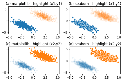

채점기준: (b)와 (d)의 그림을 seaborn으로 생성하지 않을 경우 정답으로 인정안함

(2) plotnine을 이용하여 아래와 같이 시각화하라. - alpha=0.1을 사용

x=np.concatenate([x1,x2])
y=np.concatenate([y1,y2])
df = pd.DataFrame({'x':x,'y':y,'cat':['A']*len(x1)+['B']*len(x2)})
ggplot(df)+geom_point(aes(x='x',y='y',color='cat'),alpha=0.1)\
+geom_smooth(aes(x='x',y='y',color='cat'))\
+geom_smooth(aes(x='x',y='y'))

/home/cgb4/anaconda3/envs/py37/lib/python3.7/site-packages/plotnine/stats/smoothers.py:311: PlotnineWarning: Confidence intervals are not yet implementedfor lowess smoothings.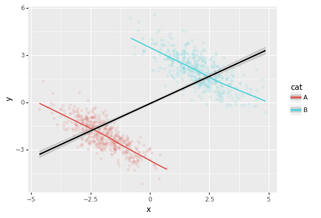

<ggplot: (8776325576381)>

채점기준: 산점도, 그룹별추세선, 전체추세선이 모두 있을 경우만 정답으로 인정

`4`. 자료분석 및 시각화 I (40점) – FIFA22자료

아래의 코드를 활용하여 FIFA22의 자료를 불러온뒤 물음에 답하라.

df = pd.read_csv('https://raw.githubusercontent.com/guebin/DV2021/master/_notebooks/2021-10-25-FIFA22_official_data.csv')
df

	ID	Name	Age	Photo	Nationality	Flag	Overall	Potential	Club	Club Logo	...	SlidingTackle	GKDiving	GKHandling	GKKicking	GKPositioning	GKReflexes	Best Position	Best Overall Rating	Release Clause	DefensiveAwareness
0	212198	Bruno Fernandes	26	https://cdn.sofifa.com/players/212/198/22_60.png	Portugal	https://cdn.sofifa.com/flags/pt.png	88	89	Manchester United	https://cdn.sofifa.com/teams/11/30.png	...	65.0	12.0	14.0	15.0	8.0	14.0	CAM	88.0	€206.9M	72.0
1	209658	L. Goretzka	26	https://cdn.sofifa.com/players/209/658/22_60.png	Germany	https://cdn.sofifa.com/flags/de.png	87	88	FC Bayern München	https://cdn.sofifa.com/teams/21/30.png	...	77.0	13.0	8.0	15.0	11.0	9.0	CM	87.0	€160.4M	74.0
2	176580	L. Suárez	34	https://cdn.sofifa.com/players/176/580/22_60.png	Uruguay	https://cdn.sofifa.com/flags/uy.png	88	88	Atlético de Madrid	https://cdn.sofifa.com/teams/240/30.png	...	38.0	27.0	25.0	31.0	33.0	37.0	ST	88.0	€91.2M	42.0
3	192985	K. De Bruyne	30	https://cdn.sofifa.com/players/192/985/22_60.png	Belgium	https://cdn.sofifa.com/flags/be.png	91	91	Manchester City	https://cdn.sofifa.com/teams/10/30.png	...	53.0	15.0	13.0	5.0	10.0	13.0	CM	91.0	€232.2M	68.0
4	224334	M. Acuña	29	https://cdn.sofifa.com/players/224/334/22_60.png	Argentina	https://cdn.sofifa.com/flags/ar.png	84	84	Sevilla FC	https://cdn.sofifa.com/teams/481/30.png	...	82.0	8.0	14.0	13.0	13.0	14.0	LB	84.0	€77.7M	80.0
...	...	...	...	...	...	...	...	...	...	...	...	...	...	...	...	...	...	...	...	...	...
16705	240558	18 L. Clayton	17	https://cdn.sofifa.com/players/240/558/18_60.png	England	https://cdn.sofifa.com/flags/gb-eng.png	53	70	Cheltenham Town	https://cdn.sofifa.com/teams/1936/30.png	...	12.0	55.0	54.0	52.0	50.0	59.0	GK	52.0	€238K	NaN
16706	262846	�. Dobre	20	https://cdn.sofifa.com/players/262/846/22_60.png	Romania	https://cdn.sofifa.com/flags/ro.png	53	63	FC Academica Clinceni	https://cdn.sofifa.com/teams/113391/30.png	...	12.0	57.0	52.0	53.0	48.0	58.0	GK	53.0	€279K	5.0
16707	241317	21 Xue Qinghao	19	https://cdn.sofifa.com/players/241/317/21_60.png	China PR	https://cdn.sofifa.com/flags/cn.png	47	60	Shanghai Shenhua FC	https://cdn.sofifa.com/teams/110955/30.png	...	9.0	49.0	48.0	45.0	38.0	52.0	GK	47.0	€223K	21.0
16708	259646	A. Shaikh	18	https://cdn.sofifa.com/players/259/646/22_60.png	India	https://cdn.sofifa.com/flags/in.png	47	67	ATK Mohun Bagan FC	https://cdn.sofifa.com/teams/113146/30.png	...	13.0	49.0	41.0	39.0	45.0	49.0	GK	47.0	€259K	7.0
16709	178453	07 A. Censori	17	https://cdn.sofifa.com/players/178/453/07_60.png	Italy	https://cdn.sofifa.com/flags/it.png	28	38	Arezzo	https://cdn.sofifa.com/teams/110907/30.png	...	NaN	7.0	1.0	36.0	6.0	9.0	ST	36.0	NaN	NaN

16710 rows × 65 columns

(1) 연령별로 선수들의 잠재력을 시각화하고 싶다. 여기에서 잠재력은 아래의 수식의 Potential2를 의미한다.

Potential2 = Potential - Overall

아래의 세부지침에 맞추어 연령별 Potential2의 산점도와 boxplot을 그려라. – (10점)

(세부지침)

step1: 결측치가 가장 많은 2개의 컬럼을 찾고 이를 제거하라.

step2: dropna()를 이용하여 결측치를 제거하라.

step3: Potential2 = Potential - Overall 를 이용하여 Potential2를 구하라.

step4: 구간 [0,20,22,26,100]를 설정하고 이를 기준으로 Age를 그룹화하라. (총 4개의 그룹으로 나누어져야 한다)

step5: 그룹화된 Age를 x축으로, Potential2를 y축으로, 색깔을 그룹화된 Age로 설정한 뒤 산점도와 박스플랏을 겹쳐그려라. - 산점도의 파라메터: alpha=0.5,size=0.1,position=‘jitter’ - 박스플랏의 파라메터: alpha=0.8

(풀이)

df.info()

<class 'pandas.core.frame.DataFrame'>
RangeIndex: 16710 entries, 0 to 16709
Data columns (total 65 columns):
 #   Column                    Non-Null Count  Dtype  
---  ------                    --------------  -----  
 0   ID                        16710 non-null  int64  
 1   Name                      16710 non-null  object 
 2   Age                       16710 non-null  int64  
 3   Photo                     16710 non-null  object 
 4   Nationality               16710 non-null  object 
 5   Flag                      16710 non-null  object 
 6   Overall                   16710 non-null  int64  
 7   Potential                 16710 non-null  int64  
 8   Club                      16446 non-null  object 
 9   Club Logo                 16710 non-null  object 
 10  Value                     16710 non-null  object 
 11  Wage                      16710 non-null  object 
 12  Special                   16710 non-null  int64  
 13  Preferred Foot            16710 non-null  object 
 14  International Reputation  16710 non-null  float64
 15  Weak Foot                 16710 non-null  float64
 16  Skill Moves               16710 non-null  float64
 17  Work Rate                 16710 non-null  object 
 18  Body Type                 16681 non-null  object 
 19  Real Face                 16681 non-null  object 
 20  Position                  16684 non-null  object 
 21  Jersey Number             16684 non-null  float64
 22  Joined                    15198 non-null  object 
 23  Loaned From               1132 non-null   object 
 24  Contract Valid Until      16359 non-null  object 
 25  Height                    16710 non-null  object 
 26  Weight                    16710 non-null  object 
 27  Crossing                  16710 non-null  float64
 28  Finishing                 16710 non-null  float64
 29  HeadingAccuracy           16710 non-null  float64
 30  ShortPassing              16710 non-null  float64
 31  Volleys                   16673 non-null  float64
 32  Dribbling                 16710 non-null  float64
 33  Curve                     16673 non-null  float64
 34  FKAccuracy                16710 non-null  float64
 35  LongPassing               16710 non-null  float64
 36  BallControl               16710 non-null  float64
 37  Acceleration              16710 non-null  float64
 38  SprintSpeed               16710 non-null  float64
 39  Agility                   16673 non-null  float64
 40  Reactions                 16710 non-null  float64
 41  Balance                   16673 non-null  float64
 42  ShotPower                 16710 non-null  float64
 43  Jumping                   16673 non-null  float64
 44  Stamina                   16710 non-null  float64
 45  Strength                  16710 non-null  float64
 46  LongShots                 16710 non-null  float64
 47  Aggression                16710 non-null  float64
 48  Interceptions             16702 non-null  float64
 49  Positioning               16702 non-null  float64
 50  Vision                    16673 non-null  float64
 51  Penalties                 16710 non-null  float64
 52  Composure                 16459 non-null  float64
 53  Marking                   892 non-null    float64
 54  StandingTackle            16710 non-null  float64
 55  SlidingTackle             16673 non-null  float64
 56  GKDiving                  16710 non-null  float64
 57  GKHandling                16710 non-null  float64
 58  GKKicking                 16710 non-null  float64
 59  GKPositioning             16710 non-null  float64
 60  GKReflexes                16710 non-null  float64
 61  Best Position             16710 non-null  object 
 62  Best Overall Rating       16710 non-null  float64
 63  Release Clause            14961 non-null  object 
 64  DefensiveAwareness        15818 non-null  float64
dtypes: float64(40), int64(5), object(20)
memory usage: 8.3+ MB

’Loaned From’와 ’Marking’이 가장 결측치가 많이 포함되어있음

data1= df.drop(columns=['Loaned From', 'Marking']).dropna()\
.eval('Potential2 = Potential- Overall')\
.assign(Age = lambda df: pd.cut(df['Age'],[0,20,22,26,100]))
data1

	ID	Name	Age	Photo	Nationality	Flag	Overall	Potential	Club	Club Logo	...	GKDiving	GKHandling	GKKicking	GKPositioning	GKReflexes	Best Position	Best Overall Rating	Release Clause	DefensiveAwareness	Potential2
0	212198	Bruno Fernandes	(22, 26]	https://cdn.sofifa.com/players/212/198/22_60.png	Portugal	https://cdn.sofifa.com/flags/pt.png	88	89	Manchester United	https://cdn.sofifa.com/teams/11/30.png	...	12.0	14.0	15.0	8.0	14.0	CAM	88.0	€206.9M	72.0	1
1	209658	L. Goretzka	(22, 26]	https://cdn.sofifa.com/players/209/658/22_60.png	Germany	https://cdn.sofifa.com/flags/de.png	87	88	FC Bayern München	https://cdn.sofifa.com/teams/21/30.png	...	13.0	8.0	15.0	11.0	9.0	CM	87.0	€160.4M	74.0	1
2	176580	L. Suárez	(26, 100]	https://cdn.sofifa.com/players/176/580/22_60.png	Uruguay	https://cdn.sofifa.com/flags/uy.png	88	88	Atlético de Madrid	https://cdn.sofifa.com/teams/240/30.png	...	27.0	25.0	31.0	33.0	37.0	ST	88.0	€91.2M	42.0	0
3	192985	K. De Bruyne	(26, 100]	https://cdn.sofifa.com/players/192/985/22_60.png	Belgium	https://cdn.sofifa.com/flags/be.png	91	91	Manchester City	https://cdn.sofifa.com/teams/10/30.png	...	15.0	13.0	5.0	10.0	13.0	CM	91.0	€232.2M	68.0	0
4	224334	M. Acuña	(26, 100]	https://cdn.sofifa.com/players/224/334/22_60.png	Argentina	https://cdn.sofifa.com/flags/ar.png	84	84	Sevilla FC	https://cdn.sofifa.com/teams/481/30.png	...	8.0	14.0	13.0	13.0	14.0	LB	84.0	€77.7M	80.0	0
...	...	...	...	...	...	...	...	...	...	...	...	...	...	...	...	...	...	...	...	...	...
16703	259718	F. Gebhardt	(0, 20]	https://cdn.sofifa.com/players/259/718/22_60.png	Germany	https://cdn.sofifa.com/flags/de.png	52	66	FC Basel 1893	https://cdn.sofifa.com/teams/896/30.png	...	53.0	45.0	47.0	52.0	57.0	GK	52.0	€361K	6.0	14
16704	251433	B. Voll	(0, 20]	https://cdn.sofifa.com/players/251/433/22_60.png	Germany	https://cdn.sofifa.com/flags/de.png	58	69	F.C. Hansa Rostock	https://cdn.sofifa.com/teams/27/30.png	...	59.0	60.0	56.0	55.0	61.0	GK	58.0	€656K	5.0	11
16706	262846	�. Dobre	(0, 20]	https://cdn.sofifa.com/players/262/846/22_60.png	Romania	https://cdn.sofifa.com/flags/ro.png	53	63	FC Academica Clinceni	https://cdn.sofifa.com/teams/113391/30.png	...	57.0	52.0	53.0	48.0	58.0	GK	53.0	€279K	5.0	10
16707	241317	21 Xue Qinghao	(0, 20]	https://cdn.sofifa.com/players/241/317/21_60.png	China PR	https://cdn.sofifa.com/flags/cn.png	47	60	Shanghai Shenhua FC	https://cdn.sofifa.com/teams/110955/30.png	...	49.0	48.0	45.0	38.0	52.0	GK	47.0	€223K	21.0	13
16708	259646	A. Shaikh	(0, 20]	https://cdn.sofifa.com/players/259/646/22_60.png	India	https://cdn.sofifa.com/flags/in.png	47	67	ATK Mohun Bagan FC	https://cdn.sofifa.com/teams/113146/30.png	...	49.0	41.0	39.0	45.0	49.0	GK	47.0	€259K	7.0	20

14398 rows × 64 columns

fig = ggplot(data=data1)
scatter = geom_point(aes(x='Age',y='Potential2',colour='Age'),alpha=0.5,size=0.1,position='jitter')
boxplot = geom_boxplot(aes(x='Age',y='Potential2',colour='Age'),alpha=0.8)
fig+scatter+boxplot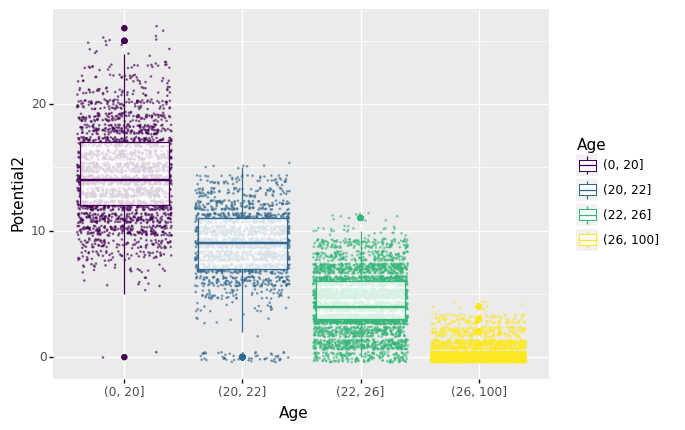

<ggplot: (8776319269061)>

채점기준: Age의 Label을 사용하지 않아도 만점으로 인정함.

(2) 포지션별로 선수들의 능력치와 Wage를 시각화하고 싶다. 아래의 dictionary를 이용하여 Position을 재정의하라.

position_dict = {
    'GOALKEEPER':{'GK'},
    'DEFENDER':{'CB','RCB','LCB','RB','LB','RWB','LWB'},
    'MIDFIELDER':{'CM','RCM','LCM','CDM','RDM','LDM','CAM','RAM','LAM','RM','LM'},
    'FORWARD':{'ST','CF','RF','LF','RW','LW','RS','LS'},
    'SUB':{'SUB'},
    'RES':{'RES'}
}
position_dict

{'GOALKEEPER': {'GK'},
 'DEFENDER': {'CB', 'LB', 'LCB', 'LWB', 'RB', 'RCB', 'RWB'},
 'MIDFIELDER': {'CAM',
  'CDM',
  'CM',
  'LAM',
  'LCM',
  'LDM',
  'LM',
  'RAM',
  'RCM',
  'RDM',
  'RM'},
 'FORWARD': {'CF', 'LF', 'LS', 'LW', 'RF', 'RS', 'RW', 'ST'},
 'SUB': {'SUB'},
 'RES': {'RES'}}

아래의 세부지침에 맞추어 포지션별 ShotPower와 SlidingTackle의 산점도를 그려라. – (30점)

세부지침

step1: 결측치가 가장 많은 2개의 컬럼을 찾고 이를 제거하라.

step2: dropna()를 이용하여 결측치를 제거하라.

step3: hint1과 position_dict을 참고하여 Position을 적절하게 변환하라. (변환된 값을 Position으로 저장할 것)

step4: hint2를 참고하여 Wage를 적절하게 변환하라. (변환된 값을 Wage에 저장할 것)

step5: Position==“DEFENDER” or Position==“FORWARD”에 해당하는 관측치를 고른 뒤 x축에 ShotPower, y축에 SlidingTackle 을 시각화하라. Position은 color로 구분하고 Wage는 size와 alpha로 구분하라.

hint1: Position column의 변환을 위한 코드

'<span class="pos pos18">CAM'.split('>')

['<span class="pos pos18"', 'CAM']

hint2: Wage column의 변환을 위한 함수

def f(x):
    if x[-1] == 'K' :
        y= float(x[1:-1])*1000
    elif x[-1] == 'M' : 
        y= float(x[1:-1])*1000000
    else:
        y= 0 
    return y

(풀이)

data2=df.drop(columns=['Loaned From', 'Marking']).dropna()\
.assign(Wage = lambda df: list(map(f,df['Wage'])))\
.assign(Position = lambda df: list(map(lambda x: x.split('>')[-1], df.Position)))\
.assign(Position = lambda df: 
        [key for x in df.Position for key in position_dict if x in position_dict[key]]
       )
data2

	ID	Name	Age	Photo	Nationality	Flag	Overall	Potential	Club	Club Logo	...	SlidingTackle	GKDiving	GKHandling	GKKicking	GKPositioning	GKReflexes	Best Position	Best Overall Rating	Release Clause	DefensiveAwareness
0	212198	Bruno Fernandes	26	https://cdn.sofifa.com/players/212/198/22_60.png	Portugal	https://cdn.sofifa.com/flags/pt.png	88	89	Manchester United	https://cdn.sofifa.com/teams/11/30.png	...	65.0	12.0	14.0	15.0	8.0	14.0	CAM	88.0	€206.9M	72.0
1	209658	L. Goretzka	26	https://cdn.sofifa.com/players/209/658/22_60.png	Germany	https://cdn.sofifa.com/flags/de.png	87	88	FC Bayern München	https://cdn.sofifa.com/teams/21/30.png	...	77.0	13.0	8.0	15.0	11.0	9.0	CM	87.0	€160.4M	74.0
2	176580	L. Suárez	34	https://cdn.sofifa.com/players/176/580/22_60.png	Uruguay	https://cdn.sofifa.com/flags/uy.png	88	88	Atlético de Madrid	https://cdn.sofifa.com/teams/240/30.png	...	38.0	27.0	25.0	31.0	33.0	37.0	ST	88.0	€91.2M	42.0
3	192985	K. De Bruyne	30	https://cdn.sofifa.com/players/192/985/22_60.png	Belgium	https://cdn.sofifa.com/flags/be.png	91	91	Manchester City	https://cdn.sofifa.com/teams/10/30.png	...	53.0	15.0	13.0	5.0	10.0	13.0	CM	91.0	€232.2M	68.0
4	224334	M. Acuña	29	https://cdn.sofifa.com/players/224/334/22_60.png	Argentina	https://cdn.sofifa.com/flags/ar.png	84	84	Sevilla FC	https://cdn.sofifa.com/teams/481/30.png	...	82.0	8.0	14.0	13.0	13.0	14.0	LB	84.0	€77.7M	80.0
...	...	...	...	...	...	...	...	...	...	...	...	...	...	...	...	...	...	...	...	...	...
16703	259718	F. Gebhardt	19	https://cdn.sofifa.com/players/259/718/22_60.png	Germany	https://cdn.sofifa.com/flags/de.png	52	66	FC Basel 1893	https://cdn.sofifa.com/teams/896/30.png	...	10.0	53.0	45.0	47.0	52.0	57.0	GK	52.0	€361K	6.0
16704	251433	B. Voll	20	https://cdn.sofifa.com/players/251/433/22_60.png	Germany	https://cdn.sofifa.com/flags/de.png	58	69	F.C. Hansa Rostock	https://cdn.sofifa.com/teams/27/30.png	...	10.0	59.0	60.0	56.0	55.0	61.0	GK	58.0	€656K	5.0
16706	262846	�. Dobre	20	https://cdn.sofifa.com/players/262/846/22_60.png	Romania	https://cdn.sofifa.com/flags/ro.png	53	63	FC Academica Clinceni	https://cdn.sofifa.com/teams/113391/30.png	...	12.0	57.0	52.0	53.0	48.0	58.0	GK	53.0	€279K	5.0
16707	241317	21 Xue Qinghao	19	https://cdn.sofifa.com/players/241/317/21_60.png	China PR	https://cdn.sofifa.com/flags/cn.png	47	60	Shanghai Shenhua FC	https://cdn.sofifa.com/teams/110955/30.png	...	9.0	49.0	48.0	45.0	38.0	52.0	GK	47.0	€223K	21.0
16708	259646	A. Shaikh	18	https://cdn.sofifa.com/players/259/646/22_60.png	India	https://cdn.sofifa.com/flags/in.png	47	67	ATK Mohun Bagan FC	https://cdn.sofifa.com/teams/113146/30.png	...	13.0	49.0	41.0	39.0	45.0	49.0	GK	47.0	€259K	7.0

14398 rows × 63 columns

fig = ggplot(data=data2.query('Position=="DEFENDER" or Position=="FORWARD"'))
scatter = geom_point(aes(x='ShotPower',y='SlidingTackle',color='Position',size='Wage',alpha='Wage'))
fig+scatter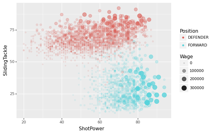

<ggplot: (8776325574701)>

채점기준: df[‘Position’]이 아니라 df[‘Best Position’]을 이용하여 자료를 변형하고 시각화 하는 경우 부분점수 없이 0점임

`5`. 자료분석 및 시각화 II (20점) – HRDataset_v14

아래의 코드를 활용하여 Kaggle의 HRdataset을 불러오고 물음에 답하라.

df = pd.read_csv('https://raw.githubusercontent.com/guebin/DV2022/master/posts/HRDataset_v14.csv')
df

	Employee_Name	EmpID	MarriedID	MaritalStatusID	GenderID	EmpStatusID	DeptID	PerfScoreID	FromDiversityJobFairID	Salary	...	ManagerName	ManagerID	RecruitmentSource	PerformanceScore	EngagementSurvey	EmpSatisfaction	SpecialProjectsCount	LastPerformanceReview_Date	DaysLateLast30	Absences
0	Adinolfi, Wilson K	10026	0	0	1	1	5	4	0	62506	...	Michael Albert	22.0	LinkedIn	Exceeds	4.60	5	0	1/17/2019	0	1
1	Ait Sidi, Karthikeyan	10084	1	1	1	5	3	3	0	104437	...	Simon Roup	4.0	Indeed	Fully Meets	4.96	3	6	2/24/2016	0	17
2	Akinkuolie, Sarah	10196	1	1	0	5	5	3	0	64955	...	Kissy Sullivan	20.0	LinkedIn	Fully Meets	3.02	3	0	5/15/2012	0	3
3	Alagbe,Trina	10088	1	1	0	1	5	3	0	64991	...	Elijiah Gray	16.0	Indeed	Fully Meets	4.84	5	0	1/3/2019	0	15
4	Anderson, Carol	10069	0	2	0	5	5	3	0	50825	...	Webster Butler	39.0	Google Search	Fully Meets	5.00	4	0	2/1/2016	0	2
...	...	...	...	...	...	...	...	...	...	...	...	...	...	...	...	...	...	...	...	...	...
306	Woodson, Jason	10135	0	0	1	1	5	3	0	65893	...	Kissy Sullivan	20.0	LinkedIn	Fully Meets	4.07	4	0	2/28/2019	0	13
307	Ybarra, Catherine	10301	0	0	0	5	5	1	0	48513	...	Brannon Miller	12.0	Google Search	PIP	3.20	2	0	9/2/2015	5	4
308	Zamora, Jennifer	10010	0	0	0	1	3	4	0	220450	...	Janet King	2.0	Employee Referral	Exceeds	4.60	5	6	2/21/2019	0	16
309	Zhou, Julia	10043	0	0	0	1	3	3	0	89292	...	Simon Roup	4.0	Employee Referral	Fully Meets	5.00	3	5	2/1/2019	0	11
310	Zima, Colleen	10271	0	4	0	1	5	3	0	45046	...	David Stanley	14.0	LinkedIn	Fully Meets	4.50	5	0	1/30/2019	0	2

311 rows × 36 columns

(1) 데이터를 조사하고 올바르게 분석한 사람을 모두 고르라. (모두 맞칠경우만 정답으로 인정)

소윤: 근무인원수가 가장 많은 인종(RaceDesc)은 ’White’이며 이는 ’Asian’인종과 ’Black or African American’의 합보다 많다.
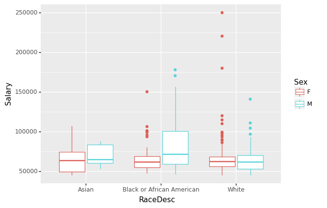
다호: ’RaceDesc==White’의 성별(Sex)임금차이는 2000이상이다.
하니: 퇴직한사람(Termd==1)은 모두 104명이며 백인여성의 퇴직자수가 가장 많다.
도한: 퇴직한사람중 아시아인의 비율은 10%가 넘지 않는다.

(풀이)

모두 참이다.

데이터조사

df.info()

<class 'pandas.core.frame.DataFrame'>
RangeIndex: 311 entries, 0 to 310
Data columns (total 36 columns):
 #   Column                      Non-Null Count  Dtype  
---  ------                      --------------  -----  
 0   Employee_Name               311 non-null    object 
 1   EmpID                       311 non-null    int64  
 2   MarriedID                   311 non-null    int64  
 3   MaritalStatusID             311 non-null    int64  
 4   GenderID                    311 non-null    int64  
 5   EmpStatusID                 311 non-null    int64  
 6   DeptID                      311 non-null    int64  
 7   PerfScoreID                 311 non-null    int64  
 8   FromDiversityJobFairID      311 non-null    int64  
 9   Salary                      311 non-null    int64  
 10  Termd                       311 non-null    int64  
 11  PositionID                  311 non-null    int64  
 12  Position                    311 non-null    object 
 13  State                       311 non-null    object 
 14  Zip                         311 non-null    int64  
 15  DOB                         311 non-null    object 
 16  Sex                         311 non-null    object 
 17  MaritalDesc                 311 non-null    object 
 18  CitizenDesc                 311 non-null    object 
 19  HispanicLatino              311 non-null    object 
 20  RaceDesc                    311 non-null    object 
 21  DateofHire                  311 non-null    object 
 22  DateofTermination           104 non-null    object 
 23  TermReason                  311 non-null    object 
 24  EmploymentStatus            311 non-null    object 
 25  Department                  311 non-null    object 
 26  ManagerName                 311 non-null    object 
 27  ManagerID                   303 non-null    float64
 28  RecruitmentSource           311 non-null    object 
 29  PerformanceScore            311 non-null    object 
 30  EngagementSurvey            311 non-null    float64
 31  EmpSatisfaction             311 non-null    int64  
 32  SpecialProjectsCount        311 non-null    int64  
 33  LastPerformanceReview_Date  311 non-null    object 
 34  DaysLateLast30              311 non-null    int64  
 35  Absences                    311 non-null    int64  
dtypes: float64(2), int64(16), object(18)
memory usage: 87.6+ KB

EmpID가 missing이 없는 열임

소윤: 근무인원수가 가장 많은 인종(RaceDesc)은 ’White’이며 이는 ’Asian’인종과 ’Black or African American’의 합보다 많다. — 참

df.groupby(by='RaceDesc').agg({'EmpID':len})

	EmpID
RaceDesc
American Indian or Alaska Native	3
Asian	29
Black or African American	80
Hispanic	1
Two or more races	11
White	187

29+80

다호: ’RaceDesc==White’의 성별(Sex)임금차이는 2000이상이다. — 참

df.groupby(by=['RaceDesc','Sex']).agg({'Salary':np.mean})

		Salary
RaceDesc	Sex
American Indian or Alaska Native	F	63436.500000
American Indian or Alaska Native	M	70545.000000
Asian	F	67520.117647
Asian	M	69939.416667
Black or African American	F	66963.829787
Black or African American	M	85066.121212
Hispanic	M	83667.000000
Two or more races	F	58068.500000
Two or more races	M	62313.800000
White	F	68846.519231
White	M	65334.132530

68846.519231 - 65334.132530

3512.386700999996

하니: 퇴직한사람(Termd==1)은 모두 104명이며 백인여성의 퇴직자수가 가장 많다. — 참

(df.Termd==1).sum()

df.groupby(by=['RaceDesc','Sex']).agg({'Termd':np.sum})

		Termd
RaceDesc	Sex
American Indian or Alaska Native	F	0
American Indian or Alaska Native	M	0
Asian	F	6
Asian	M	3
Black or African American	F	15
Black or African American	M	14
Hispanic	M	0
Two or more races	F	2
Two or more races	M	1
White	F	37
White	M	26

도한: 퇴직한사람중 아시아인의 비율은 10%가 넘지 않는다. — 참

(df.Termd==1).sum()

df.groupby(by=['RaceDesc']).agg({'Termd':np.sum})

	Termd
RaceDesc
American Indian or Alaska Native	0
Asian	9
Black or African American	29
Hispanic	0
Two or more races	3
White	63

9/104

0.08653846153846154

(2) White, Black or African American, Asian 인종(RaceDesc)에 대하여 남여급여차이를 조사하고자 한다. 아래와 같은 Boxplot을 생성하라.

(풀이)

ggplot(data=df.query('RaceDesc == "White" or RaceDesc == "Black or African American" or RaceDesc == "Asian"'))\
+geom_boxplot(aes(x='RaceDesc',y='Salary',color='Sex'))

<ggplot: (8776333683953)>

1. 시각화의 해석 - 다음을 잘 읽고 물음에 답하라. (20점)

2. 시각화구현 I - 다음을 잘 읽고 물음에 답하라. (10점)

3. 시각화구현 II – 다음을 잘 읽고 물음에 답하라. (10점)

4. 자료분석 및 시각화 I (40점) – FIFA22자료

5. 자료분석 및 시각화 II (20점) – HRDataset_v14

`1`. 시각화의 해석 - 다음을 잘 읽고 물음에 답하라. (20점)

`2`. 시각화구현 I - 다음을 잘 읽고 물음에 답하라. (10점)

`3`. 시각화구현 II – 다음을 잘 읽고 물음에 답하라. (10점)

`4`. 자료분석 및 시각화 I (40점) – FIFA22자료

`5`. 자료분석 및 시각화 II (20점) – HRDataset_v14