판다스– 인덱싱(2), 판다스–새로운열의할당(1), 아이스크림을 많이 먹으면 걸리는 병(1)

강의영상

https://youtube.com/playlist?list=PLQqh36zP38-yjgL4NsZ1NVQm_xXrrZzBA

imports

import numpy as np
import pandas as pd
import matplotlib.pyplot as plt

판다스: 인덱싱 3단계– column의 선택 (with 실전예제)

- 지금까지 정리

	`.`	`[]`	`.iloc`	`.loc`
row/단일레이블	X	X	O	O
col/단일레이블	O	O	O	O
row/레이블리스트	X	X	O	O
col/레이블리스트	X	O	O	O
row/슬라이싱	X	O	O	O
col/슬라이싱	X	X	O	O
row/bool,list	X	O	O	O
row/bool,ser	X	O	X	O
row/bool,map	X	X	O	O
col/bool,list	X	?	?	?
col/bool,ser	X	?	?	?
col/bool,map	X	?	?	?

- 채워보세요 (숙제입니다) –> 그냥 제가 채웠어요

	`.`	`[]`	`.iloc`	`.loc`	commnets
row/단일레이블	X	X	O	O
col/단일레이블	O	O	O	O
row/레이블리스트	X	X	O	O
col/레이블리스트	X	O	O	O
row/슬라이싱	X	O	O	O
col/슬라이싱	X	X	O	O
row/bool,list	X	O	O	O
row/bool,ser	X	O	X	O
row/bool,map	X	X	O	O
col/bool,list	X	X	O	O
col/bool,ser	X	X	X	X	쓸일이없음
col/bool,map	X	X	O	O

데이터

df=pd.read_csv('https://raw.githubusercontent.com/PacktPublishing/Pandas-Cookbook/master/data/movie.csv')
df

	color	director_name	num_critic_for_reviews	duration	director_facebook_likes	actor_3_facebook_likes	actor_2_name	actor_1_facebook_likes	gross	genres	...	num_user_for_reviews	language	country	content_rating	budget	title_year	actor_2_facebook_likes	imdb_score	aspect_ratio	movie_facebook_likes
0	Color	James Cameron	723.0	178.0	0.0	855.0	Joel David Moore	1000.0	760505847.0	Action\|Adventure\|Fantasy\|Sci-Fi	...	3054.0	English	USA	PG-13	237000000.0	2009.0	936.0	7.9	1.78	33000
1	Color	Gore Verbinski	302.0	169.0	563.0	1000.0	Orlando Bloom	40000.0	309404152.0	Action\|Adventure\|Fantasy	...	1238.0	English	USA	PG-13	300000000.0	2007.0	5000.0	7.1	2.35	0
2	Color	Sam Mendes	602.0	148.0	0.0	161.0	Rory Kinnear	11000.0	200074175.0	Action\|Adventure\|Thriller	...	994.0	English	UK	PG-13	245000000.0	2015.0	393.0	6.8	2.35	85000
3	Color	Christopher Nolan	813.0	164.0	22000.0	23000.0	Christian Bale	27000.0	448130642.0	Action\|Thriller	...	2701.0	English	USA	PG-13	250000000.0	2012.0	23000.0	8.5	2.35	164000
4	NaN	Doug Walker	NaN	NaN	131.0	NaN	Rob Walker	131.0	NaN	Documentary	...	NaN	NaN	NaN	NaN	NaN	NaN	12.0	7.1	NaN	0
...	...	...	...	...	...	...	...	...	...	...	...	...	...	...	...	...	...	...	...	...	...
4911	Color	Scott Smith	1.0	87.0	2.0	318.0	Daphne Zuniga	637.0	NaN	Comedy\|Drama	...	6.0	English	Canada	NaN	NaN	2013.0	470.0	7.7	NaN	84
4912	Color	NaN	43.0	43.0	NaN	319.0	Valorie Curry	841.0	NaN	Crime\|Drama\|Mystery\|Thriller	...	359.0	English	USA	TV-14	NaN	NaN	593.0	7.5	16.00	32000
4913	Color	Benjamin Roberds	13.0	76.0	0.0	0.0	Maxwell Moody	0.0	NaN	Drama\|Horror\|Thriller	...	3.0	English	USA	NaN	1400.0	2013.0	0.0	6.3	NaN	16
4914	Color	Daniel Hsia	14.0	100.0	0.0	489.0	Daniel Henney	946.0	10443.0	Comedy\|Drama\|Romance	...	9.0	English	USA	PG-13	NaN	2012.0	719.0	6.3	2.35	660
4915	Color	Jon Gunn	43.0	90.0	16.0	16.0	Brian Herzlinger	86.0	85222.0	Documentary	...	84.0	English	USA	PG	1100.0	2004.0	23.0	6.6	1.85	456

4916 rows × 28 columns

- 열의 이름을 출력하여 보자.

기본인덱싱 (df 인덱싱공부 1단계 내용)

- color ~ num_voted_user 를 뽑고 + aspect_ratio 도 추가적으로 뽑고싶다. -> loc으로는 못하겠어요..

df.loc[:,['color':'num_voted_users','aspect_ratio']]

SyntaxError: invalid syntax (1210972629.py, line 1)

- (팁) 복잡한 조건은 iloc으로 쓰는게 편할때가 있다. \(\to\) 그런데 df.columns 변수들이 몇번인지 알아보기 힘듬 \(\to\) 아래와 같이 하면 열의 이름을 인덱스와 함께 출력할 수 있음

pd.Series(df.columns)

0                         color
1                 director_name
2        num_critic_for_reviews
3                      duration
4       director_facebook_likes
5        actor_3_facebook_likes
6                  actor_2_name
7        actor_1_facebook_likes
8                         gross
9                        genres
10                 actor_1_name
11                  movie_title
12              num_voted_users
13    cast_total_facebook_likes
14                 actor_3_name
15         facenumber_in_poster
16                plot_keywords
17              movie_imdb_link
18         num_user_for_reviews
19                     language
20                      country
21               content_rating
22                       budget
23                   title_year
24       actor_2_facebook_likes
25                   imdb_score
26                 aspect_ratio
27         movie_facebook_likes
dtype: object

list(range(13))+[26]

[0, 1, 2, 3, 4, 5, 6, 7, 8, 9, 10, 11, 12, 26]

df.iloc[:,list(range(13))+[26]]

	color	director_name	num_critic_for_reviews	duration	director_facebook_likes	actor_3_facebook_likes	actor_2_name	actor_1_facebook_likes	gross	genres	actor_1_name	movie_title	num_voted_users	aspect_ratio
0	Color	James Cameron	723.0	178.0	0.0	855.0	Joel David Moore	1000.0	760505847.0	Action\|Adventure\|Fantasy\|Sci-Fi	CCH Pounder	Avatar	886204	1.78
1	Color	Gore Verbinski	302.0	169.0	563.0	1000.0	Orlando Bloom	40000.0	309404152.0	Action\|Adventure\|Fantasy	Johnny Depp	Pirates of the Caribbean: At World's End	471220	2.35
2	Color	Sam Mendes	602.0	148.0	0.0	161.0	Rory Kinnear	11000.0	200074175.0	Action\|Adventure\|Thriller	Christoph Waltz	Spectre	275868	2.35
3	Color	Christopher Nolan	813.0	164.0	22000.0	23000.0	Christian Bale	27000.0	448130642.0	Action\|Thriller	Tom Hardy	The Dark Knight Rises	1144337	2.35
4	NaN	Doug Walker	NaN	NaN	131.0	NaN	Rob Walker	131.0	NaN	Documentary	Doug Walker	Star Wars: Episode VII - The Force Awakens	8	NaN
...	...	...	...	...	...	...	...	...	...	...	...	...	...	...
4911	Color	Scott Smith	1.0	87.0	2.0	318.0	Daphne Zuniga	637.0	NaN	Comedy\|Drama	Eric Mabius	Signed Sealed Delivered	629	NaN
4912	Color	NaN	43.0	43.0	NaN	319.0	Valorie Curry	841.0	NaN	Crime\|Drama\|Mystery\|Thriller	Natalie Zea	The Following	73839	16.00
4913	Color	Benjamin Roberds	13.0	76.0	0.0	0.0	Maxwell Moody	0.0	NaN	Drama\|Horror\|Thriller	Eva Boehnke	A Plague So Pleasant	38	NaN
4914	Color	Daniel Hsia	14.0	100.0	0.0	489.0	Daniel Henney	946.0	10443.0	Comedy\|Drama\|Romance	Alan Ruck	Shanghai Calling	1255	2.35
4915	Color	Jon Gunn	43.0	90.0	16.0	16.0	Brian Herzlinger	86.0	85222.0	Documentary	John August	My Date with Drew	4285	1.85

4916 rows × 14 columns

actor라는 단어가 포함된 column 선택

- 다시 열의 이름들을 확인

df.columns

Index(['color', 'director_name', 'num_critic_for_reviews', 'duration',
       'director_facebook_likes', 'actor_3_facebook_likes', 'actor_2_name',
       'actor_1_facebook_likes', 'gross', 'genres', 'actor_1_name',
       'movie_title', 'num_voted_users', 'cast_total_facebook_likes',
       'actor_3_name', 'facenumber_in_poster', 'plot_keywords',
       'movie_imdb_link', 'num_user_for_reviews', 'language', 'country',
       'content_rating', 'budget', 'title_year', 'actor_2_facebook_likes',
       'imdb_score', 'aspect_ratio', 'movie_facebook_likes'],
      dtype='object')

- 방법1

df.iloc[:,list(map(lambda x : 'actor' in x, df.columns) )]

	actor_3_facebook_likes	actor_2_name	actor_1_facebook_likes	actor_1_name	actor_3_name	actor_2_facebook_likes
0	855.0	Joel David Moore	1000.0	CCH Pounder	Wes Studi	936.0
1	1000.0	Orlando Bloom	40000.0	Johnny Depp	Jack Davenport	5000.0
2	161.0	Rory Kinnear	11000.0	Christoph Waltz	Stephanie Sigman	393.0
3	23000.0	Christian Bale	27000.0	Tom Hardy	Joseph Gordon-Levitt	23000.0
4	NaN	Rob Walker	131.0	Doug Walker	NaN	12.0
...	...	...	...	...	...	...
4911	318.0	Daphne Zuniga	637.0	Eric Mabius	Crystal Lowe	470.0
4912	319.0	Valorie Curry	841.0	Natalie Zea	Sam Underwood	593.0
4913	0.0	Maxwell Moody	0.0	Eva Boehnke	David Chandler	0.0
4914	489.0	Daniel Henney	946.0	Alan Ruck	Eliza Coupe	719.0
4915	16.0	Brian Herzlinger	86.0	John August	Jon Gunn	23.0

4916 rows × 6 columns

- 방법2

df.loc[:,list(map(lambda x : 'actor' in x, df.columns) )]

	actor_3_facebook_likes	actor_2_name	actor_1_facebook_likes	actor_1_name	actor_3_name	actor_2_facebook_likes
0	855.0	Joel David Moore	1000.0	CCH Pounder	Wes Studi	936.0
1	1000.0	Orlando Bloom	40000.0	Johnny Depp	Jack Davenport	5000.0
2	161.0	Rory Kinnear	11000.0	Christoph Waltz	Stephanie Sigman	393.0
3	23000.0	Christian Bale	27000.0	Tom Hardy	Joseph Gordon-Levitt	23000.0
4	NaN	Rob Walker	131.0	Doug Walker	NaN	12.0
...	...	...	...	...	...	...
4911	318.0	Daphne Zuniga	637.0	Eric Mabius	Crystal Lowe	470.0
4912	319.0	Valorie Curry	841.0	Natalie Zea	Sam Underwood	593.0
4913	0.0	Maxwell Moody	0.0	Eva Boehnke	David Chandler	0.0
4914	489.0	Daniel Henney	946.0	Alan Ruck	Eliza Coupe	719.0
4915	16.0	Brian Herzlinger	86.0	John August	Jon Gunn	23.0

4916 rows × 6 columns

- 방법3

df.iloc[:,map(lambda x : 'actor' in x, df.columns)]

	actor_3_facebook_likes	actor_2_name	actor_1_facebook_likes	actor_1_name	actor_3_name	actor_2_facebook_likes
0	855.0	Joel David Moore	1000.0	CCH Pounder	Wes Studi	936.0
1	1000.0	Orlando Bloom	40000.0	Johnny Depp	Jack Davenport	5000.0
2	161.0	Rory Kinnear	11000.0	Christoph Waltz	Stephanie Sigman	393.0
3	23000.0	Christian Bale	27000.0	Tom Hardy	Joseph Gordon-Levitt	23000.0
4	NaN	Rob Walker	131.0	Doug Walker	NaN	12.0
...	...	...	...	...	...	...
4911	318.0	Daphne Zuniga	637.0	Eric Mabius	Crystal Lowe	470.0
4912	319.0	Valorie Curry	841.0	Natalie Zea	Sam Underwood	593.0
4913	0.0	Maxwell Moody	0.0	Eva Boehnke	David Chandler	0.0
4914	489.0	Daniel Henney	946.0	Alan Ruck	Eliza Coupe	719.0
4915	16.0	Brian Herzlinger	86.0	John August	Jon Gunn	23.0

4916 rows × 6 columns

- 방법4

df.loc[:,map(lambda x : 'actor' in x, df.columns)]

	actor_3_facebook_likes	actor_2_name	actor_1_facebook_likes	actor_1_name	actor_3_name	actor_2_facebook_likes
0	855.0	Joel David Moore	1000.0	CCH Pounder	Wes Studi	936.0
1	1000.0	Orlando Bloom	40000.0	Johnny Depp	Jack Davenport	5000.0
2	161.0	Rory Kinnear	11000.0	Christoph Waltz	Stephanie Sigman	393.0
3	23000.0	Christian Bale	27000.0	Tom Hardy	Joseph Gordon-Levitt	23000.0
4	NaN	Rob Walker	131.0	Doug Walker	NaN	12.0
...	...	...	...	...	...	...
4911	318.0	Daphne Zuniga	637.0	Eric Mabius	Crystal Lowe	470.0
4912	319.0	Valorie Curry	841.0	Natalie Zea	Sam Underwood	593.0
4913	0.0	Maxwell Moody	0.0	Eva Boehnke	David Chandler	0.0
4914	489.0	Daniel Henney	946.0	Alan Ruck	Eliza Coupe	719.0
4915	16.0	Brian Herzlinger	86.0	John August	Jon Gunn	23.0

4916 rows × 6 columns

s로 끝나는 column 선택

- 방법1

df.iloc[:,map(lambda x: 's' == x[-1],df.columns )]

	num_critic_for_reviews	director_facebook_likes	actor_3_facebook_likes	actor_1_facebook_likes	gross	genres	num_voted_users	cast_total_facebook_likes	plot_keywords	num_user_for_reviews	actor_2_facebook_likes	movie_facebook_likes
0	723.0	0.0	855.0	1000.0	760505847.0	Action\|Adventure\|Fantasy\|Sci-Fi	886204	4834	avatar\|future\|marine\|native\|paraplegic	3054.0	936.0	33000
1	302.0	563.0	1000.0	40000.0	309404152.0	Action\|Adventure\|Fantasy	471220	48350	goddess\|marriage ceremony\|marriage proposal\|pi...	1238.0	5000.0	0
2	602.0	0.0	161.0	11000.0	200074175.0	Action\|Adventure\|Thriller	275868	11700	bomb\|espionage\|sequel\|spy\|terrorist	994.0	393.0	85000
3	813.0	22000.0	23000.0	27000.0	448130642.0	Action\|Thriller	1144337	106759	deception\|imprisonment\|lawlessness\|police offi...	2701.0	23000.0	164000
4	NaN	131.0	NaN	131.0	NaN	Documentary	8	143	NaN	NaN	12.0	0
...	...	...	...	...	...	...	...	...	...	...	...	...
4911	1.0	2.0	318.0	637.0	NaN	Comedy\|Drama	629	2283	fraud\|postal worker\|prison\|theft\|trial	6.0	470.0	84
4912	43.0	NaN	319.0	841.0	NaN	Crime\|Drama\|Mystery\|Thriller	73839	1753	cult\|fbi\|hideout\|prison escape\|serial killer	359.0	593.0	32000
4913	13.0	0.0	0.0	0.0	NaN	Drama\|Horror\|Thriller	38	0	NaN	3.0	0.0	16
4914	14.0	0.0	489.0	946.0	10443.0	Comedy\|Drama\|Romance	1255	2386	NaN	9.0	719.0	660
4915	43.0	16.0	16.0	86.0	85222.0	Documentary	4285	163	actress name in title\|crush\|date\|four word tit...	84.0	23.0	456

4916 rows × 12 columns

- 방법2

df.loc[:,map(lambda x: 's' == x[-1],df.columns )]

	num_critic_for_reviews	director_facebook_likes	actor_3_facebook_likes	actor_1_facebook_likes	gross	genres	num_voted_users	cast_total_facebook_likes	plot_keywords	num_user_for_reviews	actor_2_facebook_likes	movie_facebook_likes
0	723.0	0.0	855.0	1000.0	760505847.0	Action\|Adventure\|Fantasy\|Sci-Fi	886204	4834	avatar\|future\|marine\|native\|paraplegic	3054.0	936.0	33000
1	302.0	563.0	1000.0	40000.0	309404152.0	Action\|Adventure\|Fantasy	471220	48350	goddess\|marriage ceremony\|marriage proposal\|pi...	1238.0	5000.0	0
2	602.0	0.0	161.0	11000.0	200074175.0	Action\|Adventure\|Thriller	275868	11700	bomb\|espionage\|sequel\|spy\|terrorist	994.0	393.0	85000
3	813.0	22000.0	23000.0	27000.0	448130642.0	Action\|Thriller	1144337	106759	deception\|imprisonment\|lawlessness\|police offi...	2701.0	23000.0	164000
4	NaN	131.0	NaN	131.0	NaN	Documentary	8	143	NaN	NaN	12.0	0
...	...	...	...	...	...	...	...	...	...	...	...	...
4911	1.0	2.0	318.0	637.0	NaN	Comedy\|Drama	629	2283	fraud\|postal worker\|prison\|theft\|trial	6.0	470.0	84
4912	43.0	NaN	319.0	841.0	NaN	Crime\|Drama\|Mystery\|Thriller	73839	1753	cult\|fbi\|hideout\|prison escape\|serial killer	359.0	593.0	32000
4913	13.0	0.0	0.0	0.0	NaN	Drama\|Horror\|Thriller	38	0	NaN	3.0	0.0	16
4914	14.0	0.0	489.0	946.0	10443.0	Comedy\|Drama\|Romance	1255	2386	NaN	9.0	719.0	660
4915	43.0	16.0	16.0	86.0	85222.0	Documentary	4285	163	actress name in title\|crush\|date\|four word tit...	84.0	23.0	456

4916 rows × 12 columns

c 혹은 d로 시작하는 column 선택

- 방법1

df.iloc[:,map(lambda x: 'c' == x[0] or 'd' == x[0] ,df.columns )]

	color	director_name	duration	director_facebook_likes	cast_total_facebook_likes	country	content_rating
0	Color	James Cameron	178.0	0.0	4834	USA	PG-13
1	Color	Gore Verbinski	169.0	563.0	48350	USA	PG-13
2	Color	Sam Mendes	148.0	0.0	11700	UK	PG-13
3	Color	Christopher Nolan	164.0	22000.0	106759	USA	PG-13
4	NaN	Doug Walker	NaN	131.0	143	NaN	NaN
...	...	...	...	...	...	...	...
4911	Color	Scott Smith	87.0	2.0	2283	Canada	NaN
4912	Color	NaN	43.0	NaN	1753	USA	TV-14
4913	Color	Benjamin Roberds	76.0	0.0	0	USA	NaN
4914	Color	Daniel Hsia	100.0	0.0	2386	USA	PG-13
4915	Color	Jon Gunn	90.0	16.0	163	USA	PG

4916 rows × 7 columns

- 방법2

df.loc[:,map(lambda x: 'c' == x[0] or 'd' == x[0] ,df.columns )]

	color	director_name	duration	director_facebook_likes	cast_total_facebook_likes	country	content_rating
0	Color	James Cameron	178.0	0.0	4834	USA	PG-13
1	Color	Gore Verbinski	169.0	563.0	48350	USA	PG-13
2	Color	Sam Mendes	148.0	0.0	11700	UK	PG-13
3	Color	Christopher Nolan	164.0	22000.0	106759	USA	PG-13
4	NaN	Doug Walker	NaN	131.0	143	NaN	NaN
...	...	...	...	...	...	...	...
4911	Color	Scott Smith	87.0	2.0	2283	Canada	NaN
4912	Color	NaN	43.0	NaN	1753	USA	TV-14
4913	Color	Benjamin Roberds	76.0	0.0	0	USA	NaN
4914	Color	Daniel Hsia	100.0	0.0	2386	USA	PG-13
4915	Color	Jon Gunn	90.0	16.0	163	USA	PG

4916 rows × 7 columns

판다스: 새로운 열의 할당 1단계

방법1: concat

df = pd.DataFrame({'a':[1,2,3],'b':[2,3,4]})
df

	a	b
0	1	2
1	2	3
2	3	4

_df = pd.DataFrame({'c':[3,4,5]}) 
_df

	c
0	3
1	4
2	5

pd.concat([df,_df],axis=1)

	a	b	c
0	1	2	3
1	2	3	4
2	3	4	5

방법2: 4가지 컨셉에 따른 할당

`#` 컨셉1: 불가능

df = pd.DataFrame({'a':[1,2,3],'b':[2,3,4]})
df

	a	b
0	1	2
1	2	3
2	3	4

df.c = pd.Series([1,2,3]) 
df

/home/cgb4/anaconda3/envs/py37/lib/python3.7/site-packages/ipykernel_launcher.py:1: UserWarning: Pandas doesn't allow columns to be created via a new attribute name - see https://pandas.pydata.org/pandas-docs/stable/indexing.html#attribute-access
  """Entry point for launching an IPython kernel.

	a	b
0	1	2
1	2	3
2	3	4

`#` 컨셉2: 가능

(예시1)

df = pd.DataFrame({'a':[1,2,3],'b':[2,3,4]})
df

	a	b
0	1	2
1	2	3
2	3	4

df['c']=[3,4,5]
df

	a	b	c
0	1	2	3
1	2	3	4
2	3	4	5

(예시2)

df = pd.DataFrame({'a':[1,2,3],'b':[2,3,4]})
df

	a	b
0	1	2
1	2	3
2	3	4

df[['c','d']]=np.array([[3,4,5],[4,5,6]]).T # 굳이.. 
df

	a	b	c	d
0	1	2	3	4
1	2	3	4	5
2	3	4	5	6

(예시3)

df = pd.DataFrame({'a':[1,2,3],'b':[2,3,4]})
df

	a	b
0	1	2
1	2	3
2	3	4

df['c'],df['d']=[3,4,5],[4,5,6]
df

	a	b	c	d
0	1	2	3	4
1	2	3	4	5
2	3	4	5	6

`#` 컨셉3: 불가능

(예시1)

df = pd.DataFrame({'a':[1,2,3],'b':[2,3,4]})
df

	a	b
0	1	2
1	2	3
2	3	4

df.iloc[:,2] = [3,4,5] 
df

IndexError: iloc cannot enlarge its target object

`#` 컨셉4: 가능

(예시1)

df = pd.DataFrame({'a':[1,2,3],'b':[2,3,4]})
df

	a	b
0	1	2
1	2	3
2	3	4

df.loc[:,'c'] = [3,4,5] 
df

	a	b	c
0	1	2	3
1	2	3	4
2	3	4	5

(예시2)

df = pd.DataFrame({'a':[1,2,3],'b':[2,3,4]})
df

	a	b
0	1	2
1	2	3
2	3	4

df.loc[:,['c','d']] = np.array([[3,4,5],[4,5,6]]).T # 이거 솔직히 되는지 몰랐어요.. 
df

	a	b	c	d
0	1	2	3	4
1	2	3	4	5
2	3	4	5	6

(예시3)

df = pd.DataFrame({'a':[1,2,3],'b':[2,3,4]})
df

	a	b
0	1	2
1	2	3
2	3	4

df.loc[:,'c'],df.loc[:,'d'] = [3,4,5],[4,5,6] 
df

	a	b	c	d
0	1	2	3	4
1	2	3	4	5
2	3	4	5	6

방법3: `.assign`으로 할당 (\(\star\)) – 제 최애

df = pd.DataFrame({'a':[1,2,3],'b':[2,3,4]})
df

	a	b
0	1	2
1	2	3
2	3	4

df.assign(c=[3,4,5])

	a	b	c
0	1	2	3
1	2	3	4
2	3	4	5

df.assign(c=[3,4,5],d=[4,5,6])

	a	b	c	d
0	1	2	3	4
1	2	3	4	5
2	3	4	5	6

df.assign(c=[3,4,5]).assign(d=[4,5,6])

	a	b	c	d
0	1	2	3	4
1	2	3	4	5
2	3	4	5	6

방법4: `.eval`을 이용한 할당

df = pd.DataFrame({'a':[1,2,3],'b':[2,3,4]})
df

	a	b
0	1	2
1	2	3
2	3	4

df.eval('c=[3,4,5]')

	a	b	c
0	1	2	3
1	2	3	4
2	3	4	5

df.eval('c=[3,4,5]').eval('d=[4,5,6]')

	a	b	c	d
0	1	2	3	4
1	2	3	4	5
2	3	4	5	6

연습해보기

`#` 데이터프레임 생성

df=pd.DataFrame({'x':np.random.randn(1000),'y':np.random.randn(1000)})
df

	x	y
0	1.085469	-1.427839
1	-1.473272	-1.527442
2	-1.007274	-1.312202
3	1.220634	-0.474995
4	-0.101496	1.636326
...	...	...
995	-0.668557	-0.435391
996	0.455894	0.796826
997	-1.004412	1.843344
998	-2.115145	-1.971965
999	0.861141	-0.193742

1000 rows × 2 columns

`#` 새로운열 `r`을 생성하고 \(r=\sqrt{x^2 + y^2}\)를 계산

- 방법1: 브로드캐스팅

df.assign(r=np.sqrt(df.x**2 + df.y**2))

	x	y	r
0	1.085469	-1.427839	1.793590
1	-1.473272	-1.527442	2.122171
2	-1.007274	-1.312202	1.654229
3	1.220634	-0.474995	1.309796
4	-0.101496	1.636326	1.639470
...	...	...	...
995	-0.668557	-0.435391	0.797831
996	0.455894	0.796826	0.918026
997	-1.004412	1.843344	2.099229
998	-2.115145	-1.971965	2.891796
999	0.861141	-0.193742	0.882667

1000 rows × 3 columns

- 방법2: lambda + map을 이용한 개별원소 계산

df.assign(r=list(map(lambda x,y: np.sqrt(x**2+y**2), df.x,df.y)))

	x	y	r
0	1.085469	-1.427839	1.793590
1	-1.473272	-1.527442	2.122171
2	-1.007274	-1.312202	1.654229
3	1.220634	-0.474995	1.309796
4	-0.101496	1.636326	1.639470
...	...	...	...
995	-0.668557	-0.435391	0.797831
996	0.455894	0.796826	0.918026
997	-1.004412	1.843344	2.099229
998	-2.115145	-1.971965	2.891796
999	0.861141	-0.193742	0.882667

1000 rows × 3 columns

- 방법3: eval

df.eval('r=sqrt(x**2+y**2)')

	x	y	r
0	1.085469	-1.427839	1.793590
1	-1.473272	-1.527442	2.122171
2	-1.007274	-1.312202	1.654229
3	1.220634	-0.474995	1.309796
4	-0.101496	1.636326	1.639470
...	...	...	...
995	-0.668557	-0.435391	0.797831
996	0.455894	0.796826	0.918026
997	-1.004412	1.843344	2.099229
998	-2.115145	-1.971965	2.891796
999	0.861141	-0.193742	0.882667

1000 rows × 3 columns

아이스크림을 많이 먹으면 걸리는 병 (1)

- ref- 데이터 과학자의 사고법: 더 나은 선택을 위한 통계학적 통찰의 힘

구매할만한 책입니다

- 내용요약

여름 \(\to\) 수영장 \(\to\) 소아마비
여름 \(\to\) 아이스크림
아이스크림과 소아마비는 상관관계가 높다: 아이스크림 성분중에서 소아마비를 유발하는 유해물질이 있을 것이다 (?)

- 아래와 같이 모형을 간단하게 하자.

온도 \(\to\) 소아마비
온도 \(\to\) 아이스크림

Toy exam

- 교재의 예제상황은 예를들면 아래와 같다.

(숨은진짜상황1)

\[\text{아이스크림 판매량} = 20 + 2 \times \text{온도} + \epsilon\]

np.random.seed(1) 
temp= np.array([-10.2, -5.2, 0.1, 10.1, 12.2, 14.7, 
                25.4, 26.8, 28.9, 35.1, 32.2, 34.6])
eps= np.random.normal(size=12,scale=5)
icecream= 20 + temp * 2 + eps

plt.plot(temp,icecream,'.')

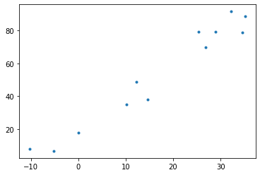
온도와 아이스크림 판매량의 산점도

(숨은진짜상황2)

\[\text{소아마비 반응수치} = 30 + 0.5 \times \text{온도} + \epsilon\] - 좌변은 소아마비임을 나타내는 어떠한 반응수치라고 생각하자.

np.random.seed(2) 
eps = np.random.normal(size=12,scale=5) 
disease = 30+ temp* 0.5 + eps

plt.plot(temp,disease,'.')

온도와 소아마비의 산점도

(우리가 데이터로부터 관측한 상황)

- 아이스크림과 질병의 산점도를 그려보자.

plt.plot(icecream,disease,'.')

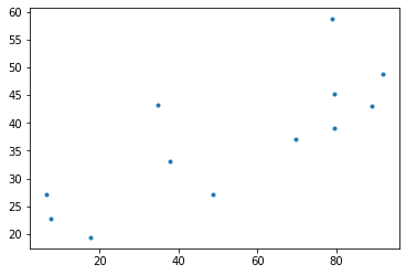
양의 상관관계에 있다.

- 아이스크림 중 어떠한 물질이 소아마비를 일으키는것이 분명하므로 (인과성이 분명해보이니까) 아래와 같은 모형을 세우자. <– 여기서부터 틀렸음

\[{\tt disease}_i =\beta_0 +\beta_1 {\tt icecream}_i +\epsilon_i,\quad \textbf{for} ~~ i=1,2,\dots, 12\]

- 적절한 \(\beta_0\)와 \(\beta_1\)을 추정하면 우리는 아이스크림과 소아마비의 관계를 알 수 있다. <– 틀린주장

틀린 모형
도데체 우리가 뭘 잘못했는가?

- 두 변수 사이에 상관관계가 있어도 실제 원인은 다른 변수에 숨겨져 있는 경우가 많다.

(ex1)

온도 \(\to\) 익사
온도 \(\to\) 아이스크림
아이스크림과 익사자도 양의 상관관계에 있을것이다.
아이스크림을 먹이면 물에 빠져 죽는다 \(\to\) 틀린주장
사실 기온이 숨겨진 원인이다. 기온이 증가하면 아이스크림 판매량도 증가하고 폭염때문에 익사사고율도 높아지는 구조이다.

(ex2)

인구수 \(\to\) 교회
인구수 \(\to\) 범죄건수
지역별 교회와 범죄건수를 살펴보면 상관관계가 높게 나올것임
교회를 지으면 범죄건수도 증가한다? \(\to\) 틀린주장
사실 인구가 숨겨진 요인임

- ex2, ex1에 대하여 바른 분석을 하려면?

ex2: 인구가 비슷한 도시끼리 묶어서 비교해보면 교회와 범죄의 건수는 양의 상관관계에 있지 않을것임
ex1: 온도가 비슷한 그룹끼리 묶어보자.

- 올바른 분석: 온도가 비슷한 그룹끼리 묶어서 그려보자. \(\to\) 상관계수가 줄어들 것이다.

plt.plot(icecream[:6],disease[:6],'.')

plt.plot(icecream[6:],disease[6:],'.')

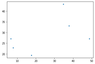
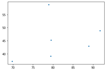
진짜로 선형관계가 약해졌다..

숙제 (수업시간에 한 내용 X)

df = pd.DataFrame({'a':[1,2,3,4],'b':[2,3,4,5],'c':[3,4,5,6],'d':[4,5,6,7]})
df

	a	b	c	d
0	1	2	3	4
1	2	3	4	5
2	3	4	5	6
3	4	5	6	7

아래의 결과를 관찰하고 drop의 기능을 유추하라.

(예시1)

df.drop(columns='a')

	b	c	d
0	2	3	4
1	3	4	5
2	4	5	6
3	5	6	7

(예시2)

df.drop(columns=['a','b'])

	c	d
0	3	4
1	4	5
2	5	6
3	6	7

(예시3)

df.drop(index=0)

	a	b	c	d
1	2	3	4	5
2	3	4	5	6
3	4	5	6	7

(예시4)

df.drop(index=range(2,4))

	a	b	c	d
0	1	2	3	4
1	2	3	4	5

문제: df 에서 a,c열을 삭제하고 첫행을 삭제하라.

#출력결과는 아래와 같아야 한다.

	b	d
1	3	5
2	4	6
3	5	7

강의영상

imports

판다스: 인덱싱 3단계– column의 선택 (with 실전예제)

데이터

기본인덱싱 (df 인덱싱공부 1단계 내용)

actor라는 단어가 포함된 column 선택

s로 끝나는 column 선택

c 혹은 d로 시작하는 column 선택

판다스: 새로운 열의 할당 1단계

방법1: concat

방법2: 4가지 컨셉에 따른 할당

# 컨셉1: 불가능

# 컨셉2: 가능

# 컨셉3: 불가능

# 컨셉4: 가능

방법3: .assign으로 할당 (\(\star\)) – 제 최애

방법4: .eval을 이용한 할당

연습해보기

# 데이터프레임 생성

# 새로운열 r을 생성하고 \(r=\sqrt{x^2 + y^2}\)를 계산

아이스크림을 많이 먹으면 걸리는 병 (1)

Toy exam

숙제 (수업시간에 한 내용 X)

`#` 컨셉1: 불가능

`#` 컨셉2: 가능

`#` 컨셉3: 불가능

`#` 컨셉4: 가능

방법3: `.assign`으로 할당 (\(\star\)) – 제 최애

방법4: `.eval`을 이용한 할당

`#` 데이터프레임 생성

`#` 새로운열 `r`을 생성하고 \(r=\sqrt{x^2 + y^2}\)를 계산