02wk-2: (회귀) – 파라메터의 학습과정 음미, MSE, 파이토치식 코딩패턴 (1)

1. 강의영상

2. Imports

import torch
import numpy as np
import matplotlib.pyplot as plt 

plt.rcParams['figure.figsize'] = (4.5, 3.0)

3. 선택학습: 데이터시각화

- 데이터시각화2023: https://guebin.github.io/DV2023/

• 01wk-2: https://guebin.github.io/DV2023/posts/01wk-2.html
• 02wk-1: https://guebin.github.io/DV2023/posts/02wk-1.html

4. 파라메터의 학습과정 음미

torch.manual_seed(43052)
x,_ = torch.randn(100).sort()
eps = torch.randn(100)*0.5
X = torch.stack([torch.ones(100),x],axis=1)
W = torch.tensor([[2.5],[4.0]])
y = X@W + eps.reshape(100,1)
x = X[:,[1]]

# 지난시간복습
# 지도학습문제: (x,y) 관찰하고 x -> y 인 패턴을 찾는 문제 (지도학습문제, supervised learning) 
# 모델링: (x,y) 관찰을 해보니까 scatter plot이 직선의 모양을 하고 있음.. --> 패턴이 직선이겠네? --> y=X@W+ϵ
## - 모델: y=X@W+ϵ // y 물결 X@W 
# 학습: 결국 회귀분석문제는 What을 찾는 문제 // 파라메터 What의 값을 update하는 과정을 학습
# 학습의방법? 
# 1. yhat을 구한다. <-- 모델링 (도메인지식이 정통한 어떤 사람) 
# 2. loss를 계산한다. <-- 손실함수를 설계 (통계) 
# 3. loss미분한다. <-- 미분을 계산하는 torch와 같은 프로그램이 있어야함 (컴퓨터공학과)
# 4. update한다. <-- 업데이트공식이 있었음. 이걸 알아야함. (산공)

A. print

What = torch.tensor([[-5.0],[10.0]],requires_grad=True)
alpha = 0.001
print(f"시작값 = {What.data.reshape(-1)}")
for epoc in range(30):
    yhat = X @ What
    loss = torch.sum((y-yhat)**2)
    loss.backward()
    What.data = What.data - alpha * What.grad
    print(f'loss = {loss:.2f} \t 업데이트폭 = {-alpha * What.grad.reshape(-1)} \t 업데이트결과: {What.data.reshape(-1)}')
    What.grad = None

시작값 = tensor([-5., 10.])
loss = 8587.69   업데이트폭 = tensor([ 1.3423, -1.1889])      업데이트결과: tensor([-3.6577,  8.8111])
loss = 5675.21   업데이트폭 = tensor([ 1.1029, -0.9499])      업데이트결과: tensor([-2.5548,  7.8612])
loss = 3755.64   업데이트폭 = tensor([ 0.9056, -0.7596])      업데이트결과: tensor([-1.6492,  7.1016])
loss = 2489.58   업데이트폭 = tensor([ 0.7431, -0.6081])      업데이트결과: tensor([-0.9061,  6.4935])
loss = 1654.04   업데이트폭 = tensor([ 0.6094, -0.4872])      업데이트결과: tensor([-0.2967,  6.0063])
loss = 1102.32   업데이트폭 = tensor([ 0.4995, -0.3907])      업데이트결과: tensor([0.2028, 5.6156])
loss = 737.84    업데이트폭 = tensor([ 0.4091, -0.3136])      업데이트결과: tensor([0.6119, 5.3020])
loss = 496.97    업데이트폭 = tensor([ 0.3350, -0.2519])      업데이트결과: tensor([0.9469, 5.0501])
loss = 337.71    업데이트폭 = tensor([ 0.2742, -0.2025])      업데이트결과: tensor([1.2211, 4.8477])
loss = 232.40    업데이트폭 = tensor([ 0.2243, -0.1629])      업데이트결과: tensor([1.4454, 4.6848])
loss = 162.73    업데이트폭 = tensor([ 0.1834, -0.1311])      업데이트결과: tensor([1.6288, 4.5537])
loss = 116.63    업데이트폭 = tensor([ 0.1500, -0.1056])      업데이트결과: tensor([1.7787, 4.4480])
loss = 86.13     업데이트폭 = tensor([ 0.1226, -0.0851])      업데이트결과: tensor([1.9013, 4.3629])
loss = 65.93     업데이트폭 = tensor([ 0.1001, -0.0687])      업데이트결과: tensor([2.0014, 4.2942])
loss = 52.57     업데이트폭 = tensor([ 0.0818, -0.0554])      업데이트결과: tensor([2.0832, 4.2388])
loss = 43.72     업데이트폭 = tensor([ 0.0668, -0.0447])      업데이트결과: tensor([2.1500, 4.1941])
loss = 37.86     업데이트폭 = tensor([ 0.0545, -0.0361])      업데이트결과: tensor([2.2045, 4.1579])
loss = 33.97     업데이트폭 = tensor([ 0.0445, -0.0292])      업데이트결과: tensor([2.2490, 4.1287])
loss = 31.40     업데이트폭 = tensor([ 0.0363, -0.0236])      업데이트결과: tensor([2.2853, 4.1051])
loss = 29.70     업데이트폭 = tensor([ 0.0296, -0.0191])      업데이트결과: tensor([2.3150, 4.0860])
loss = 28.57     업데이트폭 = tensor([ 0.0242, -0.0155])      업데이트결과: tensor([2.3392, 4.0705])
loss = 27.83     업데이트폭 = tensor([ 0.0197, -0.0125])      업데이트결과: tensor([2.3589, 4.0580])
loss = 27.33     업데이트폭 = tensor([ 0.0161, -0.0101])      업데이트결과: tensor([2.3750, 4.0479])
loss = 27.00     업데이트폭 = tensor([ 0.0131, -0.0082])      업데이트결과: tensor([2.3881, 4.0396])
loss = 26.79     업데이트폭 = tensor([ 0.0107, -0.0067])      업데이트결과: tensor([2.3988, 4.0330])
loss = 26.64     업데이트폭 = tensor([ 0.0087, -0.0054])      업데이트결과: tensor([2.4075, 4.0276])
loss = 26.55     업데이트폭 = tensor([ 0.0071, -0.0044])      업데이트결과: tensor([2.4146, 4.0232])
loss = 26.48     업데이트폭 = tensor([ 0.0058, -0.0035])      업데이트결과: tensor([2.4204, 4.0197])
loss = 26.44     업데이트폭 = tensor([ 0.0047, -0.0029])      업데이트결과: tensor([2.4251, 4.0168])
loss = 26.41     업데이트폭 = tensor([ 0.0038, -0.0023])      업데이트결과: tensor([2.4290, 4.0144])

B. 시각화 – yhat의 관점에서!

What = torch.tensor([[-5.0],[10.0]],requires_grad=True)
alpha = 0.001
plt.plot(x,y,'o',label = "observed")
fig = plt.gcf()
ax = fig.gca()
ax.plot(x,X@What.data,'--',color="C1")
for epoc in range(30):
    yhat = X @ What
    loss = torch.sum((y-yhat)**2)
    loss.backward()
    What.data = What.data - alpha * What.grad
    ax.plot(x,X@What.data,'--',color="C1",alpha=0.1)
    What.grad = None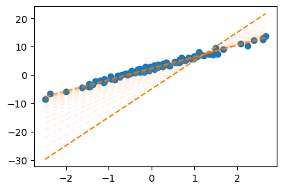

C. 시각화 – loss의 관점에서!!

def plot_loss():
    fig = plt.figure()
    ax = fig.add_subplot(projection='3d')
    w0 = np.arange(-6, 11, 0.5) 
    w1 = np.arange(-6, 11, 0.5)
    W1,W0 = np.meshgrid(w1,w0)
    LOSS=W0*0
    for i in range(len(w0)):
        for j in range(len(w1)):
            LOSS[i,j]=torch.sum((y-w0[i]-w1[j]*x)**2)
    ax.plot_surface(W0, W1, LOSS, rstride=1, cstride=1, color='b',alpha=0.1)
    ax.azim = 30  ## 3d plot의 view 조절 
    ax.dist = 8   ## 3d plot의 view 조절 
    ax.elev = 5   ## 3d plot의 view 조절 
    ax.set_xlabel(r'$w_0$')  # x축 레이블 설정
    ax.set_ylabel(r'$w_1$')  # y축 레이블 설정
    ax.set_xticks([-5,0,5,10])  # x축 틱 간격 설정
    ax.set_yticks([-5,0,5,10])  # y축 틱 간격 설정
    plt.close(fig)  # 자동 출력 방지
    return fig

# 손실 8587.6875 를 계산하는 또 다른 방식
def l(w0hat,w1hat):
    yhat = w0hat + w1hat*x
    return torch.sum((y-yhat)**2)

fig = plot_loss()
ax = fig.gca()
ax.scatter(2.5, 4, l(2.5,4), s=200, marker='*', color='red', label=r"${\bf W}=[2.5, 4]'$")
ax.scatter(-5, 10, l(-5,10), s=200, marker='*', color='blue', label=r"initial $\hat{\bf W}=[-5, 10]'$")
ax.legend()
fig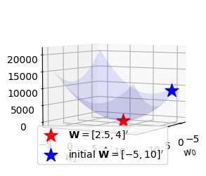

What = torch.tensor([[-5.0],[10.0]],requires_grad=True)
alpha = 0.001
for epoc in range(30):
    yhat = X @ What
    loss = torch.sum((y-yhat)**2)
    loss.backward()
    What.data = What.data - 0.001 * What.grad
    w0,w1 = What.data.reshape(-1) 
    ax.scatter(w0,w1,l(w0,w1),s=5,marker='o',color='blue')
    What.grad = None

fig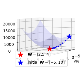

D. 애니메이션

from matplotlib import animation

plt.rcParams['figure.figsize'] = (7.5,2.5)
plt.rcParams["animation.html"] = "jshtml" 

def show_animation(alpha=0.001):
    ## 1. 히스토리 기록을 위한 list 초기화
    loss_history = [] 
    yhat_history = [] 
    What_history = [] 

    ## 2. 학습 + 학습과정기록
    What= torch.tensor([[-5.0],[10.0]],requires_grad=True)
    What_history.append(What.data.tolist())
    for epoc in range(30): 
        yhat=X@What ; yhat_history.append(yhat.data.tolist())
        loss=torch.sum((y-yhat)**2); loss_history.append(loss.item())
        loss.backward() 
        What.data = What.data - alpha * What.grad; What_history.append(What.data.tolist())
        What.grad = None    

    ## 3. 시각화 
    fig = plt.figure()
    ax1 = fig.add_subplot(1, 2, 1)
    ax2 = fig.add_subplot(1, 2, 2, projection='3d')

    #### ax1: yhat의 관점에서.. 
    ax1.plot(x,y,'o',label=r"$(x_i,y_i)$")
    line, = ax1.plot(x,yhat_history[0],label=r"$(x_i,\hat{y}_i)$") 
    ax1.legend()
    #### ax2: loss의 관점에서.. 
    w0 = np.arange(-6, 11, 0.5) 
    w1 = np.arange(-6, 11, 0.5)
    W1,W0 = np.meshgrid(w1,w0)
    LOSS=W0*0
    for i in range(len(w0)):
        for j in range(len(w1)):
            LOSS[i,j]=torch.sum((y-w0[i]-w1[j]*x)**2)
    ax2.plot_surface(W0, W1, LOSS, rstride=1, cstride=1, color='b',alpha=0.1)
    ax2.azim = 30  ## 3d plot의 view 조절 
    ax2.dist = 8   ## 3d plot의 view 조절 
    ax2.elev = 5   ## 3d plot의 view 조절 
    ax2.set_xlabel(r'$w_0$')  # x축 레이블 설정
    ax2.set_ylabel(r'$w_1$')  # y축 레이블 설정
    ax2.set_xticks([-5,0,5,10])  # x축 틱 간격 설정
    ax2.set_yticks([-5,0,5,10])  # y축 틱 간격 설정
    ax2.scatter(2.5, 4, l(2.5,4), s=200, marker='*', color='red', label=r"${\bf W}=[2.5, 4]'$")
    ax2.scatter(-5, 10, l(-5,10), s=200, marker='*', color='blue')
    ax2.legend()
    def animate(epoc):
        line.set_ydata(yhat_history[epoc])
        ax2.scatter(np.array(What_history)[epoc,0],np.array(What_history)[epoc,1],loss_history[epoc],color='grey')
        fig.suptitle(f"alpha = {alpha} / epoch = {epoc}")
        return line

    ani = animation.FuncAnimation(fig, animate, frames=30)
    plt.close()
    return ani

ani = show_animation(alpha=0.001)
ani

Once Loop Reflect

E. 학습률에 따른 시각화

- \(\alpha\)가 너무 작다면 비효율적임

show_animation(alpha=0.0001)

Once Loop Reflect

- \(\alpha\)가 크다고 무조건 좋은건 또 아님

show_animation(alpha=0.0083)

Once Loop Reflect

- 수틀리면 수렴안할수도??

show_animation(alpha=0.0085)

Once Loop Reflect

- 그냥 망할수도??

show_animation(alpha=0.01)

Once Loop Reflect

---

plt.rcdefaults()
plt.rcParams['figure.figsize'] = 4.5,3.0 

---

5. SSE \(\to\) MSE

- 학습률을 잘 선택하는 것이 중요함

- 손실함수를 SSE로 설정하면 학습률 선택이 비효율적 \(\to\) SSE말고 MSE를 써야함

손실함수가 SSE일때코드

What = torch.tensor([[-5.0],[10.0]],requires_grad = True)
for epoc in range(30):
    # step1: yhat 
    yhat = X@What 
    # step2: loss
    loss = torch.sum((y-yhat)**2)
    # step3: 미분
    loss.backward()
    # step4: update
    What.data = What.data - 0.001 * What.grad
    What.grad = None

What.data

tensor([[2.4290],
        [4.0144]])

손실함수가 MSE일때코드

What = torch.tensor([[-5.0],[10.0]],requires_grad = True)
for epoc in range(30):
    # step1: yhat 
    yhat = X@What 
    # step2: loss
    loss = torch.sum((y-yhat)**2)/100 # torch.mean((y-yhat)**2)
    # step3: 미분
    loss.backward()
    # step4: update
    What.data = What.data - 0.1 * What.grad
    What.grad = None

What.data

tensor([[2.4290],
        [4.0144]])

6. 파이토치식 코딩패턴 (1)

torch.manual_seed(43052)
x,_ = torch.randn(100).sort()
eps = torch.randn(100)*0.5
X = torch.stack([torch.ones(100),x],axis=1)
W = torch.tensor([[2.5],[4.0]])
y = X@W + eps.reshape(100,1)
x = X[:,[1]]

A. 기본패턴

## -- 외우세요!!! -- ##
What = torch.tensor([[-5.0],[10.0]],requires_grad = True)
for epoc in range(30):
    # step1: yhat 
    yhat = X@What 
    # step2: loss
    loss = torch.sum((y-yhat)**2)/100
    # step3: 미분
    loss.backward()
    # step4: update
    What.data = What.data - 0.1 * What.grad
    What.grad = None

plt.plot(x,y,'o')
plt.plot(x,X@What.data,'--')
plt.title(f'What={What.data.reshape(-1)}');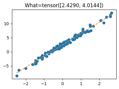

B. Step2의 수정 – loss_fn 이용

What = torch.tensor([[-5.0],[10.0]],requires_grad = True)
loss_fn = torch.nn.MSELoss()
for epoc in range(30):
    # step1: yhat 
    yhat = X@What 
    # step2: loss
    #loss = torch.sum((y-yhat)**2)/100
    loss = loss_fn(yhat,y) # 여기서는 큰 상관없지만 습관적으로 yhat을 먼저넣는 연습을 하자!!
    # step3: 미분
    loss.backward()
    # step4: update
    What.data = What.data - 0.1 * What.grad
    What.grad = None

plt.plot(x,y,'o')
plt.plot(x,X@What.data,'--')
plt.title(f'What={What.data.reshape(-1)}');

C. Step1의 수정 – net 이용

# net – net 오브젝트란?

원래 yhat을 이런식으로 구했는데 ~

What = torch.tensor([[-5.0],[10.0]],requires_grad = True)
yhat= X@What
yhat[:5]

tensor([[-29.8211],
        [-28.6215],
        [-24.9730],
        [-21.2394],
        [-19.7919]], grad_fn=<SliceBackward0>)

아래와 같은 방식으로 코드를 짜고 싶음..

yhat = net(X) # 

위와 같은 코드를 가능하게 하는 net은 torch에서 지원하고 아래와 같이 사용할 수 있음.

# yhat = net(X) 
net = torch.nn.Linear(
    in_features=2, # X:(n,2) --> 2 
    out_features=1, # yhat:(n,1) --> 1 
    bias=False 
)

net.weight.data = torch.tensor([[-5.0], [10.0]]).T # .T 를 해야함. 외우세요 
net.weight

Parameter containing:
tensor([[-5., 10.]], requires_grad=True)

net(X)[:5]

tensor([[-29.8211],
        [-28.6215],
        [-24.9730],
        [-21.2394],
        [-19.7919]], grad_fn=<SliceBackward0>)

(X@What)[:5]

tensor([[-29.8211],
        [-28.6215],
        [-24.9730],
        [-21.2394],
        [-19.7919]], grad_fn=<SliceBackward0>)

(X@net.weight.T)[:5]

tensor([[-29.8211],
        [-28.6215],
        [-24.9730],
        [-21.2394],
        [-19.7919]], grad_fn=<SliceBackward0>)

#

- 수정된코드

# step1을 위한 사전준비
net = torch.nn.Linear(
    in_features=2,
    out_features=1,
    bias=False
)
net.weight.data = torch.tensor([[-5.0,  10.0]])
# step2를 위한 사전준비
loss_fn = torch.nn.MSELoss()
for epoc in range(30):
    # step1: yhat
    # yhat = X@What 
    yhat = net(X)
    # step2: loss
    loss = loss_fn(yhat,y)
    # step3: 미분
    loss.backward()
    # step4: update
    net.weight.data = net.weight.data - 0.1 * net.weight.grad
    net.weight.grad = None

plt.plot(x,y,'o')
plt.plot(x,net(X).data,'--')
plt.title(f'net.weight={net.weight.data.reshape(-1)}');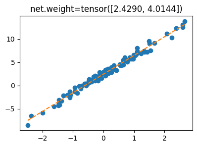

D. Step4의 수정 – optimizer의 이용

- 소망: 아래의 과정을 좀 더 편하게 했으면..

net.weight.data = net.weight.data - 0.1 * net.weight.grad
net.weight.data = None 

# optimizer – 이걸 이용하면 update 과정을 손쉽게 할 수 있음

기존코드

## -- 준비과정 -- ## 
# step1을 위한 사전준비
net = torch.nn.Linear(
    in_features=2,
    out_features=1,
    bias=False
)
net.weight.data = torch.tensor([[-5.0,  10.0]])
# step2를 위한 사전준비
loss_fn = torch.nn.MSELoss()

## -- 1에폭진행 -- ## 
# step1: 
yhat = net(X)
# step2: loss
loss = loss_fn(yhat,y)
# step3: 미분
loss.backward()
# step4: update
print(net.weight.data)
net.weight.data = net.weight.data - 0.1 * net.weight.grad
print(net.weight.data)
net.weight.grad = None

tensor([[-5., 10.]])
tensor([[-3.6577,  8.8111]])

## -- 2에폭진행 -- ## 
# step1: 2에폭진행
yhat = net(X)
# step2: loss
loss = loss_fn(yhat,y)
# step3: 미분
loss.backward()
# step4: update
print(net.weight.data)
net.weight.data = net.weight.data - 0.1 * net.weight.grad
print(net.weight.data)
net.weight.grad = None

tensor([[-3.6577,  8.8111]])
tensor([[-2.5548,  7.8612]])

새로운코드 – optimizer 이용

## -- 준비과정 -- ## 
# step1을 위한 사전준비
net = torch.nn.Linear(
    in_features=2,
    out_features=1,
    bias=False
)
net.weight.data = torch.tensor([[-5.0,  10.0]])
# step2를 위한 사전준비
loss_fn = torch.nn.MSELoss()
# step4를 위한 사전준비
optimizr = torch.optim.SGD(net.parameters(),lr=0.1)

## -- 1에폭진행 -- ## 
yhat = net(X)
# step2: loss
loss = loss_fn(yhat,y)
# step3: 미분
loss.backward()
# step4: update
print(net.weight.data)
#net.weight.data = net.weight.data - 0.1 * net.weight.grad
optimizr.step()
print(net.weight.data)
#net.weight.grad = None
optimizr.zero_grad()

tensor([[-5., 10.]])
tensor([[-3.6577,  8.8111]])

## -- 2에폭진행 -- ## 
yhat = net(X)
# step2: loss
loss = loss_fn(yhat,y)
# step3: 미분
loss.backward()
# step4: update
print(net.weight.data)
#net.weight.data = net.weight.data - 0.1 * net.weight.grad
optimizr.step()
print(net.weight.data)
#net.weight.grad = None
optimizr.zero_grad()

tensor([[-3.6577,  8.8111]])
tensor([[-2.5548,  7.8612]])

#

- 수정된코드

# step1을 위한 사전준비
net = torch.nn.Linear(
    in_features=2,
    out_features=1,
    bias=False
)
net.weight.data = torch.tensor([[-5.0,  10.0]])
# step2를 위한 사전준비
loss_fn = torch.nn.MSELoss()
# step4를 위한 사전준비 
optimizr = torch.optim.SGD(net.parameters(),lr=0.1)
for epoc in range(30):
    # step1: yhat 
    yhat = net(X)
    # step2: loss
    loss = loss_fn(yhat,y)
    # step3: 미분
    loss.backward()
    # step4: update
    optimizr.step()
    optimizr.zero_grad()

plt.plot(x,y,'o')
plt.plot(x,yhat.data,'--')
plt.title(f'net.weight={net.weight.data.reshape(-1)}');