import torch
import pandas as pd
import matplotlib.pyplot as plt09wk-2: 순환신경망 (1)
순환신경망
순환신경망 intro (1)– ab예제, embedding layer
강의영상
https://youtube.com/playlist?list=PLQqh36zP38-zya4QF67x6DZfNtJRF-iPc
import
Define some funtions
- 활성화함수들
sig = torch.nn.Sigmoid()
soft = torch.nn.Softmax(dim=1)
tanh = torch.nn.Tanh()
_x = torch.linspace(-5,5,100)
plt.plot(_x,tanh(_x))
plt.title("tanh(x)", size=15)Text(0.5, 1.0, 'tanh(x)')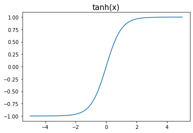
- 문자열 -> 숫자로 바꾸는 함수
def f(txt,mapping):
    return [mapping[key] for key in txt]
(사용예시1)
txt = ['a','b','a']
mapping = {'a':33,'b':-22}
print('변환전: %s'% txt)
print('변환후: %s'% f(txt,mapping))
변환전: ['a', 'b', 'a']
변환후: [33, -22, 33](사용예시2)
txt = ['a','b','a']
mapping = {'a':[1,0],'b':[0,1]}
print('변환전: %s'% txt)
print('변환후: %s'% f(txt,mapping))
변환전: ['a', 'b', 'a']
변환후: [[1, 0], [0, 1], [1, 0]]Exam1: ab
data
txt = list('ab')*100
txt[:10]
['a', 'b', 'a', 'b', 'a', 'b', 'a', 'b', 'a', 'b']txt_x = txt[:-1]
txt_y = txt[1:]txt_x[:5],txt_y[:5](['a', 'b', 'a', 'b', 'a'], ['b', 'a', 'b', 'a', 'b'])선형모형을 이용한 풀이
(풀이1) 1개의 파라메터 – 실패
- 데이터정리
x = torch.tensor(f(txt_x,{'a':0,'b':1})).float().reshape(-1,1)
y = torch.tensor(f(txt_y,{'a':0,'b':1})).float().reshape(-1,1)x[:5],y[:5](tensor([[0.],
[1.],
[0.],
[1.],
[0.]]),
tensor([[1.],
[0.],
[1.],
[0.],
[1.]]))- 학습 및 결과 시각화
net = torch.nn.Linear(in_features=1,out_features=1,bias=False)
loss_fn = torch.nn.MSELoss()
optimizr = torch.optim.Adam(net.parameters())
for epoc in range(5000):
## 1
yhat = net(x)
## 2
loss = loss_fn(yhat,y)
## 3
loss.backward()
## 4
optimizr.step()
optimizr.zero_grad()plt.plot(y[:5],'o')
plt.plot(net(x).data[:5])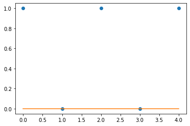
- 잘 학습이 안되었다.
- 학습이 잘 안된 이유
pd.DataFrame({'x':x[:5].reshape(-1),'y':y[:5].reshape(-1)})| x | y | |
|---|---|---|
| 0 | 0.0 | 1.0 |
| 1 | 1.0 | 0.0 |
| 2 | 0.0 | 1.0 |
| 3 | 1.0 | 0.0 |
| 4 | 0.0 | 1.0 |
현재 \(\hat{y}_i = \hat{w}x_i\) 꼴의 아키텍처이고 \(y_i \approx \hat{w}x_i\) 가 되는 적당한 \(\hat{w}\)를 찾아야 하는 상황
- \((x_i,y_i)=(0,1)\) 이면 어떠한 \(\hat{w}\)를 선택해도 \(y_i \approx \hat{w}x_i\)를 만드는 것이 불가능
- \((x_i,y_i)=(1,0)\) 이면 \(\hat{w}=0\)일 경우 \(y_i \approx \hat{w}x_i\)로 만드는 것이 가능
상황을 종합해보니 \(\hat{w}=0\)으로 학습되는 것이 그나마 최선
(풀이2) 1개의 파라메터 – 성공, but 확장성이 없는 풀이
- 0이라는 값이 문제가 되므로 인코딩방식의 변경
x = torch.tensor(f(txt_x,{'a':-1,'b':1})).float().reshape(-1,1)
y = torch.tensor(f(txt_y,{'a':-1,'b':1})).float().reshape(-1,1)x[:5],y[:5](tensor([[-1.],
[ 1.],
[-1.],
[ 1.],
[-1.]]),
tensor([[ 1.],
[-1.],
[ 1.],
[-1.],
[ 1.]]))net = torch.nn.Linear(in_features=1,out_features=1,bias=False)
loss_fn = torch.nn.MSELoss()
optimizr = torch.optim.Adam(net.parameters())for epoc in range(2000):
## 1
yhat = net(x)
## 2
loss = loss_fn(yhat,y)
## 3
loss.backward()
## 4
optimizr.step()
optimizr.zero_grad()- 결과는 성공
plt.plot(y[:5],'o')
plt.plot(net(x).data[:5])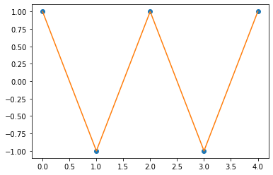
- 딱봐도 클래스가 3개일 경우 확장이 어려워 보인다.
로지스틱 모형을 이용한 풀이
(풀이1) 1개의 파라메터 – 실패
- 데이터를 다시 a=0, b=1로 정리
mapping = {'a':0,'b':1}
x = torch.tensor(f(txt_x,mapping)).float().reshape(-1,1)
y = torch.tensor(f(txt_y,mapping)).float().reshape(-1,1)x[:5],y[:5](tensor([[0.],
[1.],
[0.],
[1.],
[0.]]),
tensor([[1.],
[0.],
[1.],
[0.],
[1.]]))- 학습
net = torch.nn.Linear(in_features=1,out_features=1,bias=False)
loss_fn = torch.nn.BCEWithLogitsLoss()
optimizr = torch.optim.Adam(net.parameters())for epoc in range(5000):
## 1
yhat = net(x)
## 2
loss = loss_fn(yhat,y)
## 3
loss.backward()
## 4
optimizr.step()
optimizr.zero_grad()- 결과
plt.plot(y[:10],'o')
plt.plot(sig(net(x)).data[:10],'--o')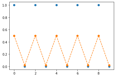
- 결과해석: 예상되었던 실패임
- 아키텍처는 \(\hat{y}_i = \text{sig}(\hat{w}x_i)\) 꼴이다.
- \((x_i,y_i)=(0,1)\) 이라면 어떠한 \(\hat{w}\)을 선택해도 \(\hat{w}x_i=0\) 이다. 이경우 \(\hat{y}_i = \text{sig}(0) = 0.5\) 가 된다.
- \((x_i,y_i)=(1,0)\) 이라면 \(\hat{w}=-5\)와 같은 값으로 선택하면 \(\text{sig}(-5) \approx 0 = y_i\) 와 같이 만들 수 있다.
- 상황을 종합하면 net의 weight는 \(\text{sig}(\hat{w}x_i) \approx 0\) 이 되도록 적당한 음수로 학습되는 것이 최선임을 알 수 있다.
net.weight # 적당한 음수값으로 학습되어있음을 확인Parameter containing:
tensor([[-4.0070]], requires_grad=True)(풀이2) 2개의 파라메터 + 좋은 초기값 – 성공
- 동일하게 a=0, b=1로 맵핑
mapping = {'a':0,'b':1}
x = torch.tensor(f(txt_x,mapping)).float().reshape(-1,1)
y = torch.tensor(f(txt_y,mapping)).float().reshape(-1,1)x[:5],y[:5](tensor([[0.],
[1.],
[0.],
[1.],
[0.]]),
tensor([[1.],
[0.],
[1.],
[0.],
[1.]]))- 네트워크에서 bias를 넣기로 결정함
net = torch.nn.Linear(in_features=1,out_features=1,bias=True)
loss_fn = torch.nn.BCEWithLogitsLoss()
optimizr = torch.optim.Adam(net.parameters())- net의 초기값을 설정 (이것은 좋은 초기값임)
net.weight.data = torch.tensor([[-5.00]])
net.bias.data = torch.tensor([+2.500])net(x)[:10]tensor([[ 2.5000],
[-2.5000],
[ 2.5000],
[-2.5000],
[ 2.5000],
[-2.5000],
[ 2.5000],
[-2.5000],
[ 2.5000],
[-2.5000]], grad_fn=<SliceBackward0>)- 학습전 결과
plt.plot(y[:10],'o')
plt.plot(sig(net(x)).data[:10],'--o')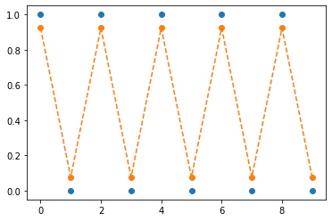
- 학습후결과
for epoc in range(5000):
    ## 1
    yhat = net(x)
    ## 2
    loss = loss_fn(yhat,y)
    ## 3
    loss.backward()
    ## 4
    optimizr.step()
optimizr.zero_grad()plt.plot(y[:10],'o')
plt.plot(sig(net(x)).data[:10],'--o')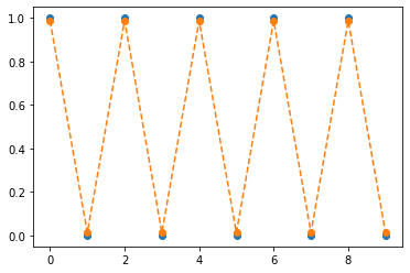
(풀이3) 2개의 파라메터 + 나쁜초기값 – 성공
- a=0, b=1
mapping = {'a':0,'b':1}
x = torch.tensor(f(txt_x,mapping)).float().reshape(-1,1)
y = torch.tensor(f(txt_y,mapping)).float().reshape(-1,1)x[:5],y[:5](tensor([[0.],
[1.],
[0.],
[1.],
[0.]]),
tensor([[1.],
[0.],
[1.],
[0.],
[1.]]))- 이전과 동일하게 바이어스가 포함된 네트워크 설정
net = torch.nn.Linear(in_features=1,out_features=1,bias=True)
loss_fn = torch.nn.BCEWithLogitsLoss()
optimizr = torch.optim.Adam(net.parameters())- 초기값설정 (이 초기값은 나쁜 초기값임)
net.weight.data = torch.tensor([[+5.00]])
net.bias.data = torch.tensor([-2.500])net(x)[:10]tensor([[-2.5000],
[ 2.5000],
[-2.5000],
[ 2.5000],
[-2.5000],
[ 2.5000],
[-2.5000],
[ 2.5000],
[-2.5000],
[ 2.5000]], grad_fn=<SliceBackward0>)- 학습전상태: 반대모양으로 되어있다.
plt.plot(y[:10],'o')
plt.plot(sig(net(x)).data[:10],'--o')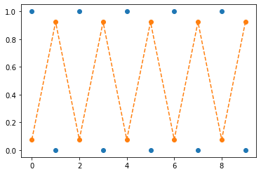
- 학습
for epoc in range(5000):
    ## 1
    yhat = net(x)
    ## 2
    loss = loss_fn(yhat,y)
    ## 3
    loss.backward()
    ## 4
    optimizr.step()
optimizr.zero_grad()plt.plot(y[:10],'o')
plt.plot(sig(net(x)).data[:10],'--o')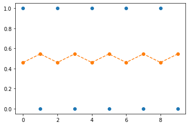
- 결국 수렴하긴 할듯
(풀이4) 3개의 파라메터를 쓴다면?
- a=0, b=1로 코딩
mapping = {'a':0,'b':1}
x = torch.tensor(f(txt_x,mapping)).float().reshape(-1,1)
y = torch.tensor(f(txt_y,mapping)).float().reshape(-1,1)x[:5],y[:5](tensor([[0.],
[1.],
[0.],
[1.],
[0.]]),
tensor([[1.],
[0.],
[1.],
[0.],
[1.]]))- 3개의 파라메터를 사용하기 위해서 아래와 같은 구조를 생각하자.
torch.nn.Sequential(
torch.nn.Linear(in_features=1,out_features=1,bias=True),
torch.nn.ACTIVATION_FUNCTION(),
torch.nn.Linear(in_features=1,out_features=1,bias=False)
)위와 같은 네트워크를 설정하면 3개의 파라메터를 사용할 수 있다. 적절한 ACTIVATION_FUNCTION을 골라야 하는데 실험적으로 tanh가 적절하다고 알려져있다. (\(\to\) 그래서 우리도 실험적으로 이해해보자)
(예비학습1) net(x)와 사실 net.forwardx(x)는 같다.
net(x)[:5] # 풀이3에서 학습한 네트워크임tensor([[-0.1584],
[ 0.1797],
[-0.1584],
[ 0.1797],
[-0.1584]], grad_fn=<SliceBackward0>)net.forward(x)[:5] # 풀이3에서 학습한 네트워크임tensor([[-0.1584],
[ 0.1797],
[-0.1584],
[ 0.1797],
[-0.1584]], grad_fn=<SliceBackward0>)그래서 net.forward를 재정의하면 net(x)의 기능을 재정의 할 수 있다.
net.forward = lambda x: 1 - “lambda x: 1” 은 입력이 x 출력이 1인 함수를 의미 (즉 입력값에 상관없이 항상 1을 출력하는 함수)
- “net.forward = lambda x:1” 이라고 새롭게 선언하였므로 앞으론 net.forward(x), net(x) 도 입력값에 상관없이 항상 1을 출력하게 될 것임
net(x)1(예비학습2) torch.nn.Module을 상속받아서 네트워크를 만들면 (= “class XXX(torch.nn.Module):” 와 같은 방식으로 클래스를 선언하면) 약속된 아키텍처를 가진 네트워크를 찍어내는 함수를 만들 수 있다.
(예시1)
class Mynet1(torch.nn.Module):
def __init__(self):
super().__init__()
self.l1 = torch.nn.Linear(in_features=1,out_features=1,bias=True)
self.a1 = torch.nn.Sigmoid()
self.l2 = torch.nn.Linear(in_features=1,out_features=1,bias=False)
def forward(self,x):
yhat = self.l2(self.a1(self.l1(x)))
return yhat이제
net = Mynet1()는 아래와 같은 효과를 가진다.
net = torch.nn.Sequential(
torch.nn.Linear(in_features=1,out_features=1,bias=True),
torch.nn.Sigmoid(),
torch.nn.Linear(in_features=1,out_features=1,bias=False)
)(예시2)
class Mynet2(torch.nn.Module):
def __init__(self):
super().__init__()
self.l1 = torch.nn.Linear(in_features=1,out_features=1,bias=True)
self.a1 = torch.nn.ReLU()
self.l2 = torch.nn.Linear(in_features=1,out_features=1,bias=False)
def forward(self,x):
yhat = self.l2(self.a1(self.l1(x)))
return yhat이제
net = Mynet2()는 아래와 같은 효과를 가진다.
net = torch.nn.Sequential(
torch.nn.Linear(in_features=1,out_features=1,bias=True),
torch.nn.RuLU(),
torch.nn.Linear(in_features=1,out_features=1,bias=False)
)(예시3)
class Mynet3(torch.nn.Module):
def __init__(self):
super().__init__()
self.l1 = torch.nn.Linear(in_features=1,out_features=1,bias=True)
self.a1 = torch.nn.Tanh()
self.l2 = torch.nn.Linear(in_features=1,out_features=1,bias=False)
def forward(self,x):
yhat = self.l2(self.a1(self.l1(x)))
return yhat이제
net = Mynet3()는 아래와 같은 효과를 가진다.
net = torch.nn.Sequential(
torch.nn.Linear(in_features=1,out_features=1,bias=True),
torch.nn.Tanh(),
torch.nn.Linear(in_features=1,out_features=1,bias=False)
)클래스에 대한 이해가 부족한 학생을 위한 암기방법
step1: 아래와 코드를 복사하여 틀을 만든다. (이건 무조건 고정임, XXXX 자리는 원하는 이름을 넣는다)
class XXXX(torch.nn.Module):
def __init__(self):
super().__init__()
## 우리가 사용할 레이어를 정의
## 레이어 정의 끝
def forward(self,x):
## yhat을 어떻게 구할것인지 정의
## 정의 끝
return yhat- net(x)에 사용하는 x임, yhat은 net.forward(x) 함수의 리턴값임
- 사실, x/yhat은 다른 변수로 써도 무방하나 (예를들면 input/output 이라든지) 설명의 편의상 x와 yhat을 고정한다.
step2: def __init__(self):에 사용할 레이어를 정의하고 이름을 붙인다. 이름은 항상 self.xxx 와 같은 식으로 정의한다.
class XXXX(torch.nn.Module):
def __init__(self):
super().__init__()
## 우리가 사용할 레이어를 정의
self.xxx1 = torch.nn.Linear(in_features=1,out_features=1,bias=True)
self.xxx2 = torch.nn.Tanh()
self.xxx3 = torch.nn.Linear(in_features=1,out_features=1,bias=True)
## 레이어 정의 끝
def forward(self,x):
## yhat을 어떻게 구할것인지 정의
## 정의 끝
return yhatstep3: def forward:에 “x –> yhat” 으로 가는 과정을 묘사한 코드를 작성하고 yhat을 리턴하도록 한다.
class XXXX(torch.nn.Module):
def __init__(self):
super().__init__()
## 우리가 사용할 레이어를 정의
self.xxx1 = torch.nn.Linear(in_features=1,out_features=1,bias=True)
self.xxx2 = torch.nn.Tanh()
self.xxx3 = torch.nn.Linear(in_features=1,out_features=1,bias=True)
## 레이어 정의 끝
def forward(self,x):
## yhat을 어떻게 구할것인지 정의
u = self.xxx1(x)
v = self.xxx2(u)
yhat = self.xxx3(v)
## 정의 끝
return yhat예비학습 끝
- 우리가 하려고 했던 것: 아래의 아키텍처에서
torch.nn.Sequential(
torch.nn.Linear(in_features=1,out_features=1,bias=True),
torch.nn.ACTIVATION_FUNCTION(),
torch.nn.Linear(in_features=1,out_features=1,bias=False)
)ACTIVATION의 자리에 tanh가 왜 적절한지 직관을 얻어보자.
- 실험결과1(Sig): Sigmoid activation을 포함한 아키텍처로 학습시킨 25개의 적합결과
fig, ax = plt.subplots(5,5,figsize=(10,10))
for i in range(5):
for j in range(5):
net = Mynet1()
loss_fn = torch.nn.BCEWithLogitsLoss()
optimizr = torch.optim.Adam(net.parameters())
for epoc in range(1000):
## 1
yhat = net(x)
## 2
loss = loss_fn(yhat,y)
## 3
loss.backward()
## 4
optimizr.step()
optimizr.zero_grad()
ax[i][j].plot(y[:5],'o')
ax[i][j].plot(sig(net(x[:5])).data,'--o')
fig.suptitle(r"$a_1(x):=Sigmoid(x)$",size=20)
fig.tight_layout()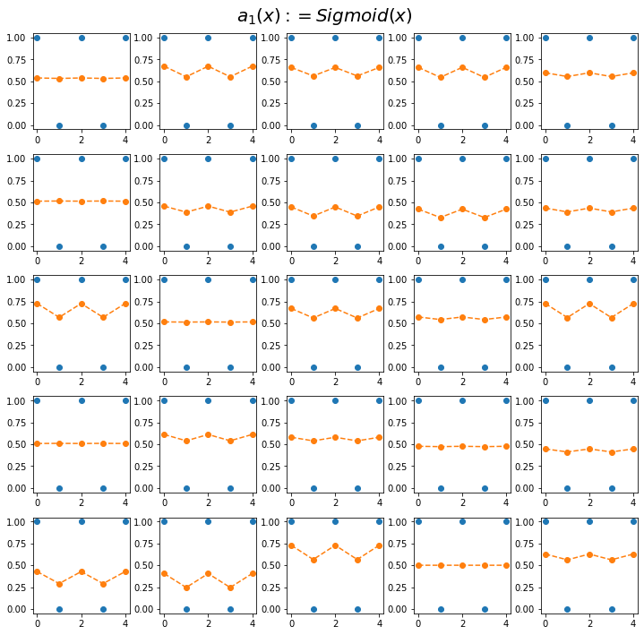
- 실험결과2(ReLU): RuLU activation을 포함한 아키텍처로 학습시킨 25개의 적합결과
fig, ax = plt.subplots(5,5,figsize=(10,10))
for i in range(5):
for j in range(5):
net = Mynet2()
loss_fn = torch.nn.BCEWithLogitsLoss()
optimizr = torch.optim.Adam(net.parameters())
for epoc in range(1000):
## 1
yhat = net(x)
## 2
loss = loss_fn(yhat,y)
## 3
loss.backward()
## 4
optimizr.step()
optimizr.zero_grad()
ax[i][j].plot(y[:5],'o')
ax[i][j].plot(sig(net(x[:5])).data,'--o')
fig.suptitle(r"$a_2(x):=ReLU(x)$",size=20)
fig.tight_layout()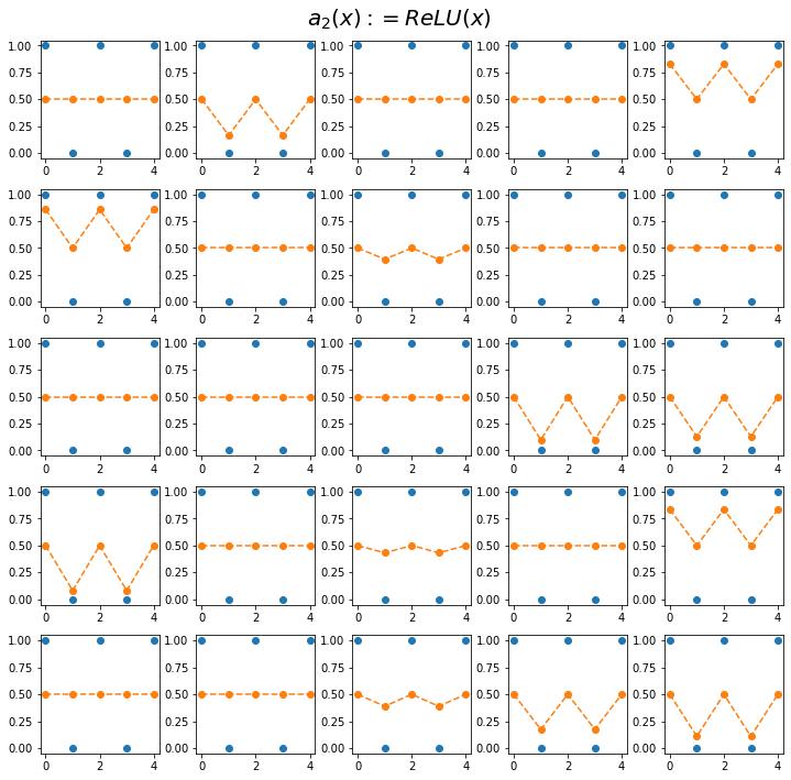
- 실험결과3(Tanh): Tanh activation을 포함한 아키텍처로 학습시킨 25개의 적합결과
fig, ax = plt.subplots(5,5,figsize=(10,10))
for i in range(5):
for j in range(5):
net = Mynet3()
loss_fn = torch.nn.BCEWithLogitsLoss()
optimizr = torch.optim.Adam(net.parameters())
for epoc in range(1000):
## 1
yhat = net(x)
## 2
loss = loss_fn(yhat,y)
## 3
loss.backward()
## 4
optimizr.step()
optimizr.zero_grad()
ax[i][j].plot(y[:5],'o')
ax[i][j].plot(sig(net(x[:5])).data,'--o')
fig.suptitle(r"$a_2(x):=Tanh(x)$",size=20)
fig.tight_layout()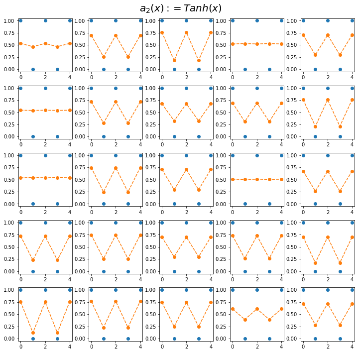
- 실험해석 - sig: 주황색선의 변동폭이 작음 + 항상 0.5근처로 머무는 적합값이 존재 - relu: 주황색선의 변동폭이 큼 + 항상 0.5근처로 머무는 적합값이 존재 - tanh: 주황색선의 변동폭이 큼 + 0.5근처로 머무는 적합값이 존재X
- 실험해보니까 tanh가 우수한것 같다. \(\to\) 앞으로는 tanh를 쓰자.
소프트맥스로 확장
(풀이1) 로지스틱모형에서 3개의 파라메터 버전을 그대로 확장
mapping = {'a':[1,0],'b':[0,1]}
x = torch.tensor(f(txt_x,mapping)).float().reshape(-1,2)
y = torch.tensor(f(txt_y,mapping)).float().reshape(-1,2)
x[:5],y[:5](tensor([[1., 0.],
[0., 1.],
[1., 0.],
[0., 1.],
[1., 0.]]),
tensor([[0., 1.],
[1., 0.],
[0., 1.],
[1., 0.],
[0., 1.]]))net = torch.nn.Sequential(
torch.nn.Linear(in_features=2,out_features=1),
torch.nn.Tanh(),
torch.nn.Linear(in_features=1,out_features=2,bias=False)
)
loss_fn = torch.nn.CrossEntropyLoss()
optimizr = torch.optim.Adam(net.parameters())for epoc in range(5000):
## 1
yhat = net(x)
## 2
loss = loss_fn(yhat,y)
## 3
loss.backward()
## 4
optimizr.step()
optimizr.zero_grad()y[:5][:,0]tensor([0., 1., 0., 1., 0.])plt.plot(y[:5][:,1],'o')
plt.plot(soft(net(x[:5]))[:,1].data,'--r')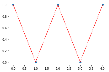
fig,ax = plt.subplots(1,2)
ax[0].imshow(y[:5])
ax[1].imshow(soft(net(x[:5])).data)<matplotlib.image.AxesImage at 0x7f2633e40f90>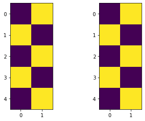
Embedding Layer
motive
- 결국 최종적으로는 아래와 같은 맵핑방식이 확장성이 있어보인다.
mapping = {'a':[1,0,0],'b':[0,1,0],'c':[0,0,1]} # 원핫인코딩 방식 - 그런데 매번 \(X\)를 원핫인코딩하고 Linear 변환하는것이 번거로운데 이를 한번에 구현하는 함수가 있으면 좋겠다. \(\to\) torch.nn.Embedding Layer가 그 역할을 한다.
mapping = {'a':0,'b':1,'c':2}
x = torch.tensor(f(list('abc')*100,mapping))
y = torch.tensor(f(list('bca')*100,mapping))
x[:5],y[:5](tensor([0, 1, 2, 0, 1]), tensor([1, 2, 0, 1, 2]))torch.manual_seed(43052)
ebdd = torch.nn.Embedding(num_embeddings=3,embedding_dim=1)ebdd(x)[:5]tensor([[-0.8178],
[-0.7052],
[-0.5843],
[-0.8178],
[-0.7052]], grad_fn=<SliceBackward0>)- 그런데 사실 언뜻보면 아래의 linr 함수와 역할의 차이가 없어보인다.
torch.manual_seed(43052)
linr = torch.nn.Linear(in_features=1,out_features=1)linr(x.float().reshape(-1,1))[:5]tensor([[-0.8470],
[-1.1937],
[-1.5404],
[-0.8470],
[-1.1937]], grad_fn=<SliceBackward0>)- 차이점: 파라메터수에 차이가 있다.
ebdd.weightParameter containing:
tensor([[-0.8178],
[-0.7052],
[-0.5843]], requires_grad=True)linr.weight, linr.bias(Parameter containing:
tensor([[-0.3467]], requires_grad=True),
Parameter containing:
tensor([-0.8470], requires_grad=True))결국 ebdd는 아래의 구조에 해당하는 파라메터들이고
- \(\text{x[:5]}= \begin{bmatrix} 0 \\ 1 \\ 2 \\ 0 \\ 1 \end{bmatrix} \Longrightarrow \begin{bmatrix} 1 & 0 & 0 \\ 0 & 1 & 0 \\ 0 & 0 & 1 \\ 1 & 0 & 0 \\ 0 & 1 & 0 \end{bmatrix} \quad net(x)= \begin{bmatrix} 1 & 0 & 0 \\ 0 & 1 & 0 \\ 0 & 0 & 1 \\ 1 & 0 & 0 \\ 0 & 1 & 0 \end{bmatrix}\begin{bmatrix} -0.8178 \\ -0.7052 \\ -0.5843 \end{bmatrix} = \begin{bmatrix} -0.8178 \\ -0.7052 \\ -0.5843 \\ -0.8178 \\ -0.7052 \end{bmatrix}\)
linr는 아래의 구조에 해당하는 파라메터이다.
- \(\text{x[:5]}= \begin{bmatrix} 0 \\ 1 \\ 2 \\ 0 \\ 1 \end{bmatrix} \quad net(x)= \begin{bmatrix} 0 \\ 1 \\ 2 \\ 0 \\ 1 \end{bmatrix} \times (-0.3467) + (-0.8470)=\begin{bmatrix} -0.8470 \\ -1.1937 \\ -1.5404 \\ -0.8470 \\ -1.1937 \end{bmatrix}\)
연습 (ab문제 소프트맥스로 확장한 것 다시 풀이)
- 맵핑
mapping = {'a':0,'b':1}
x = torch.tensor(f(txt_x,mapping))
y = torch.tensor(f(txt_y,mapping))
x[:5],y[:5](tensor([0, 1, 0, 1, 0]), tensor([1, 0, 1, 0, 1]))- torch.nn.Embedding 을 넣은 네트워크
net = torch.nn.Sequential(
torch.nn.Embedding(num_embeddings=2,embedding_dim=1),
torch.nn.Tanh(),
torch.nn.Linear(in_features=1,out_features=2)
)
loss_fn = torch.nn.CrossEntropyLoss()
optimizr = torch.optim.Adam(net.parameters())- 학습
for epoc in range(5000):
    ## 1
    yhat = net(x)
    ## 2
    loss = loss_fn(yhat,y)
    ## 3
    loss.backward()
    ## 4
    optimizr.step()
optimizr.zero_grad()plt.plot(y[:5],'o')
plt.plot(soft(net(x[:5]))[:,1].data,'--r')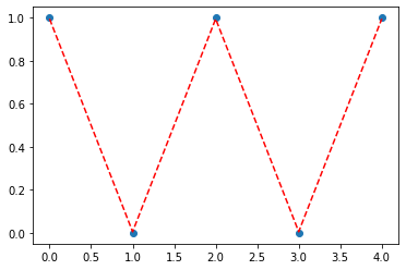
plt.imshow(soft(net(x[:5])).data)<matplotlib.image.AxesImage at 0x7f2633f7f450>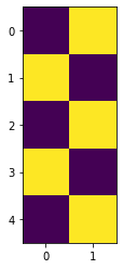
HW
아래의 코드를 관찰하라.
x = [0,1]*5
y = [1,0]*5
torch.manual_seed(43052) # 편의상 시드를 고정
ebdd = torch.nn.Embedding(num_embeddings=2,embedding_dim=1)ebdd.weightParameter containing:
tensor([[-0.8178],
[-0.7052]], requires_grad=True)ebdd(x)의 출력결과를 예측하여 작성하라.
(풀이)
굳이 실행해보지 않아도 아래임을 알 수 있다.
- \(\text{x}= \begin{bmatrix} 0 \\ 1 \\ 0 \\ 1 \\ 0 \\ 1 \\ 0 \\ 1 \\ 0 \\ 1 \end{bmatrix} \Longrightarrow \begin{bmatrix} 1 & 0 \\ 0 & 1 \\ 1 & 0 \\ 0 & 1 \\ 1 & 0 \\ 0 & 1 \\ 1 & 0 \\ 0 & 1 \\ 1 & 0 \\ 0 & 1 \end{bmatrix} \quad net(x)= \begin{bmatrix} 1 & 0 \\ 0 & 1 \\ 1 & 0 \\ 0 & 1 \\ 1 & 0 \\ 0 & 1 \\ 1 & 0 \\ 0 & 1 \\ 1 & 0 \\ 0 & 1 \end{bmatrix} \begin{bmatrix} -0.8178 \\ -0.7052 \end{bmatrix} = \begin{bmatrix} -0.8178 \\ -0.7052 \\ -0.8178 \\ -0.7052 \\-0.8178 \\ -0.7052 \\-0.8178 \\ -0.7052 \\-0.8178 \\ -0.7052 \end{bmatrix}\)
실행해보면서 확인
x = torch.tensor(x) # ebdd에 넣기위해서 x를 텐서로 변환
x
tensor([0, 1, 0, 1, 0, 1, 0, 1, 0, 1])ebdd(x)tensor([[-0.8178],
[-0.7052],
[-0.8178],
[-0.7052],
[-0.8178],
[-0.7052],
[-0.8178],
[-0.7052],
[-0.8178],
[-0.7052]], grad_fn=<EmbeddingBackward0>)