03wk-2: 딥러닝의 기초 (1)

딥러닝의 기초

Author

최규빈

Published

September 20, 2022

회귀분석(1)– 회귀모형의 소개, 회귀모형에서 데이터생성, 회귀모형에서 학습이란? 파라메터를 학습하는 방법, 파라메터의 학습과정 음미, 학습률

- 강의노트가 약간 수정되었습니다 (loss.backward()의 계산결과 검증에서 편미분의 간단한 구현을 통한 검증이 추가되었습니다)

강의영상

https://youtube.com/playlist?list=PLQqh36zP38-xQuhazVVLGdKZp2Vo-2A2L

imports

import torch
import numpy as np
import matplotlib.pyplot as plt

로드맵

- 회귀분석 $\to$ 로지스틱 $\to$ 심층신경망(DNN) $\to$ 합성곱신경망(CNN)

- 강의계획서

ref

- 넘파이 문법이 약하다면? (reshape, concatenate, stack)

reshape: 넘파이공부 2단계 reshape 참고
concatenate, stack: 아래 링크의 넘파이공부 4단계 참고

회귀모형 소개

- model: $y_i= w_0+w_1 x_i +\epsilon_i = 2.5 + 4x_i +\epsilon_i, \quad i=1,2,\dots,n$

- model: ${\bf y}={\bf X}{\bf W} +\boldsymbol{\epsilon}$

${\bf y}=\begin{bmatrix} y_1 \\ y_2 \\ \dots \\ y_n\end{bmatrix}, \quad {\bf X}=\begin{bmatrix} 1 & x_1 \\ 1 & x_2 \\ \dots \\ 1 & x_n\end{bmatrix}, \quad {\bf W}=\begin{bmatrix} 2.5 \\ 4 \end{bmatrix}, \quad \boldsymbol{\epsilon}= \begin{bmatrix} \epsilon_1 \\ \dots \\ \epsilon_n\end{bmatrix}$

회귀모형에서 데이터 생성

torch.manual_seed(43052)
ones= torch.ones(100)
x,_ = torch.randn(100).sort()
X = torch.stack([ones,x]).T # torch.stack([ones,x],axis=1)
W = torch.tensor([2.5,4])
ϵ = torch.randn(100)*0.5
y = X@W + ϵ

plt.plot(x,y,'o')
plt.plot(x,2.5+4*x,'--')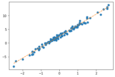

회귀모형에서 학습이란?

- 파란점만 주어졌을때, 주황색 점선을 추정하는것. 좀 더 정확하게 말하면 given data로 $\begin{bmatrix} \hat{w}_0 \\ \hat{w}_1 \end{bmatrix}$를 최대한 $\begin{bmatrix} 2.5 \\ 4 \end{bmatrix}$와 비슷하게 찾는것.

given data : $\big\{(x_i,y_i) \big\}_{i=1}^{n}$
parameter: ${\bf W}=\begin{bmatrix} w_0 \\ w_1 \end{bmatrix}$
estimated parameter: ${\bf \hat{W}}=\begin{bmatrix} \hat{w}_0 \\ \hat{w}_1 \end{bmatrix}$

- 더 쉽게 말하면 아래의 그림을 보고 적당한 추세선을 찾는것이다.

plt.plot(x,y,'o')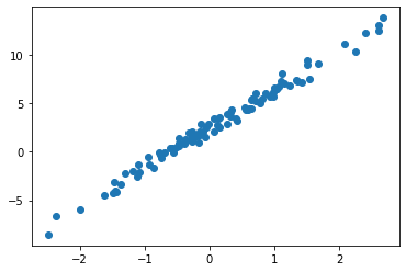

- 시도: $(\hat{w}_0,\hat{w}_1)=(-5,10)$을 선택하여 선을 그려보고 적당한지 판단.

plt.plot(x,y,'o')
plt.plot(x,-5+10*x,'--')

$\hat{y}_i=-5 +10 x_i$ 와 같이 $y_i$의 값을 적합시키겠다는 의미

- 벡터표현으로 주황색점선을 계산

What = torch.tensor([-5.0,10.0])

X.shape

torch.Size([100, 2])

plt.plot(x,y,'o')
plt.plot(x,X@What,'--')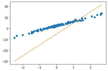

파라메터를 학습하는 방법 (적당한 선으로 업데이트 하는 방법)

- 이론적으로 추론 <- 회귀분석시간에 배운것

- 컴퓨터의 반복계산을 이용하여 추론 (손실함수도입 + 경사하강법) <- 우리가 오늘 파이토치로 실습해볼 내용.

- 전략: 아래와 같은 3단계 전략을 취한다.

stage1: 아무 점선이나 그어본다..
stage2: stage1에서 그은 점선보다 더 좋은 점선으로 바꾼다.
stage3: stage1 - 2 를 반복한다.

Stage1: 첫번째 점선 – 임의의 선을 일단 그어보자

- $\hat{w}_0=-5, \hat{w}_1 = 10$ 으로 설정하고 (왜? 그냥) 임의의 선을 그어보자.

What = torch.tensor([-5.0,10.0],requires_grad=True)
What

tensor([-5., 10.], requires_grad=True)

처음에는 ${\bf \hat{W}}=\begin{bmatrix} \hat{w}_0 \\ \hat{w}_1 \end{bmatrix}=\begin{bmatrix} -5 \\ 10 \end{bmatrix}$ 를 대입해서 주황색 점선을 적당히 그려보자는 의미
끝에 requires_grad=True는 나중에 미분을 위한 것

yhat = X@What

plt.plot(x,y,'o')
plt.plot(x,yhat.data,'--') # 그림을 그리기 위해서 yhat의 미분꼬리표를 제거

Stage2: 첫번째 수정 – 최초의 점선에 대한 ‘적당한 정도’를 판단하고 더 ’적당한’ 점선으로 업데이트 한다.

- ’적당한 정도’를 판단하기 위한 장치: loss function 도입!

$loss=\sum_{i=1}^{n}(y_i-\hat{y}_i)^2=\sum_{i=1}^{n}(y_i-(\hat{w}_0+\hat{w}_1x_i))^2$

$=({\bf y}-{\bf\hat{y}})^\top({\bf y}-{\bf\hat{y}})=({\bf y}-{\bf X}{\bf \hat{W}})^\top({\bf y}-{\bf X}{\bf \hat{W}})$

- loss 함수의 특징 - $y_i \approx \hat{y}_i$ 일수록 loss값이 작다. - $y_i \approx \hat{y}_i$ 이 되도록 $(\hat{w}_0,\hat{w}_1)$을 잘 찍으면 loss값이 작다. - (중요) 주황색 점선이 ‘적당할 수록’ loss값이 작다.

loss = torch.sum((y-yhat)**2)
loss

tensor(8587.6875, grad_fn=<SumBackward0>)

- 우리의 목표: 이 loss(=8587.6875)을 더 줄이자. - 궁극적으로는 아예 모든 조합 $(\hat{w}_0,\hat{w}_1)$에 대하여 가장 작은 loss를 찾으면 좋겠다. (stage2에서 할일은 아님)

- 문제의 치환: 생각해보니까 우리의 문제는 아래와 같이 수학적으로 단순화 되었다. - 적당해보이는 주황색 선을 찾자 $\to$ $loss(w_0,w_1)$를 최소로하는 $(w_0,w_1)$의 값을 찾자.

- 수정된 목표: $loss(w_0,w_1)$를 최소로 하는 $(w_0,w_1)$을 구하라. - 단순한 수학문제가 되었다. 마치 $loss(w)=w^2-2w+3$ 을 최소화하는 $w$를 찾으라는 것과 같음. - 즉 “적당한 선으로 업데이트 하라 = 파라메터를 학습 하라 = 손실함수를 최소화 하라”

- 우리의 무기: 경사하강법, 벡터미분

`#` Stage2를 위한 경사하강법 복습

경사하강법 아이디어 (1차원)

(step 1) 임의의 점을 찍는다.

(step 2) 그 점에서 순간기울기를 구한다. (접선) <– 미분

(step 3) 순간기울기(=미분계수)의 부호를 살펴보고 부호와 반대방향으로 움직인다.

(팁) 기울기의 절대값 크기와 비례하여 보폭(=움직이는 정도)을 조절한다.

경사하강법 아이디어 (2차원)

(step 1) 임의의 점을 찍는다.

(step 2) 그 점에서 순간기울기를 구한다. (접평면) <– 편미분

(step 3) 순간기울기(=미분계수)의 부호를 살펴보고 부호와 반대방향으로 각각 움직인다.

(팁) 기울기의 절대값 크기와 비례하여 보폭(=움직이는 정도)을 각각 조절한다.

loss를 줄이도록 ${\bf W}$를 개선하는 방법

- $수정값 원래값 - 기울어진크기(=미분계수) $

여기에서 $\alpha$는 전체적인 보폭의 크기를 결정한다. 즉 $\alpha$값이 클수록 한번의 update에 움직이는 양이 크다.

- ${\bf W} \leftarrow {\bf W} - \alpha \times \frac{\partial}{\partial {\bf W}}loss(w_0,w_1)$

마이너스의 의미: 기울기의 부호를 보고 반대방향으로 움직여라.
$\frac{\partial}{\partial {\bf W}}loss(w_0,w_1):$ 기울기의 절대값 크기와 비례하여 움직이는 정도를 조정하라.
$\alpha$의 의미: 전체적인 보폭의 속도를 조절, $\alpha$가 크면 전체적으로 빠르게 움직인다. 다리의 길이로 비유할 수 있다.

- 우리의 목표: loss=8587.6875 인데, 이걸 줄이는 것이 목표라고 했었음. 이것을 줄이는 방법이 경사하강법이다.

- 경사하강법으로 loss를 줄이기 위해서는 $\frac{\partial}{\partial {\bf W}}loss(w_0,w_1)$의 계산이 필요한데, 이를 위해서 벡터미분이 필요하다. (loss.backward()로 하면된다)

loss

tensor(8587.6875, grad_fn=<SumBackward0>)

loss.backward()

loss.backward()의 의미: loss를 미분해라! 뭘로? requires_grad=True를 가진 텐서로!!

loss=torch.sum((y-yhat)**2)= torch.sum((y-X@What)**2)
# 이었고 
What=torch.tensor([-5.0,10.0],requires_grad=True)
# 이므로 결국 What으로 미분하라는 의미. 
# 미분한 식이 나오는 것이 아니고, 
# 그 식에 (-5.0, 10.0)을 대입한 계수값이 계산됨.

- 위에서 loss.backward()의 과정은 미분을 활용하여 $(-5,10)$에서의 순간기울기를 구했다는 의미임.

- (-5,10)에서 loss의 순간기울기 값은 What.grad로 확인가능하다.

What,What.grad

(tensor([-5., 10.], requires_grad=True), tensor([-1342.2522,  1188.9305]))

이것이 의미하는건 $(-5,10)$에서의 $loss(w_0,w_1)$의 순간기울기가 $(-1342.2523, 1188.9307)$ 이라는 의미

- (확인1) loss.backward()가 미분을 잘 계산해 주는 것이 맞는가? 손계산으로 검증하여 보자.

$loss(w_0,w_1)=({\bf y}-\hat{\bf y})^\top ({\bf y}-\hat{\bf y})=({\bf y}-{\bf XW})^\top ({\bf y}-{\bf XW})$
$\frac{\partial}{\partial {\bf W} }loss(w_0,w_1)=-2{\bf X}^\top {\bf y}+2{\bf X}^\top {\bf X W}$

- 2 * X.T @ y + 2 * X.T @ X @ What

tensor([-1342.2522,  1188.9308], grad_fn=<AddBackward0>)

- (확인2) loss.backward()가 미분을 잘 계산해 주는 것이 맞는가? 편미분을 간단히 구현하여 검증하여 보자.

$\frac{\partial}{\partial {\bf W} } loss(w_0,w_1)=\begin{bmatrix}\frac{\partial}{\partial w_0} \\ \frac{\partial}{\partial w_1} \end{bmatrix}loss(w_0,w_1) =\begin{bmatrix}\frac{\partial}{\partial w_0}loss(w_0,w_1) \\ \frac{\partial}{\partial w_1}loss(w_0,w_1) \end{bmatrix}$
$\frac{\partial}{\partial w_0}loss(w_0,w_1) \approx \frac{loss(w_0+h,w_1)-loss(w_0,w_1)}{h}$
$\frac{\partial}{\partial w_1}loss(w_0,w_1) \approx \frac{loss(w_0,w_1+h)-loss(w_0,w_1)}{h}$

_lossfn = lambda w0,w1: torch.sum((y-w0-w1*x)**2)
_lossfn(-5,10)

tensor(8587.6875)

h=0.001
(_lossfn(-5+h,10) - _lossfn(-5,10))/h,  (_lossfn(-5,10+h) - _lossfn(-5,10))/h

(tensor(-1341.7968), tensor(1190.4297))

약간 오차가 있지만 얼추비슷 $\to$ 잘 계산했다는 소리임

- 수정전, 수정하는폭, 수정후의 값은 차례로 아래와 같다.

alpha=0.001 
print('수정전: ' + str(What.data)) # What 에서 미분꼬리표를 떼고 싶다면? What.data or What.detach()
print('수정하는폭: ' +str(-alpha * What.grad))
print('수정후: ' +str(What.data-alpha * What.grad))
print('*참값: (2.5,4)' )

수정전: tensor([-5., 10.])
수정하는폭: tensor([ 1.3423, -1.1889])
수정후: tensor([-3.6577,  8.8111])
*참값: (2.5,4)

- Wbefore, Wafter 계산

Wbefore = What.data
Wafter = What.data- alpha * What.grad
Wbefore, Wafter

(tensor([-5., 10.]), tensor([-3.6577,  8.8111]))

- Wbefore, Wafter의 시각화

plt.plot(x,y,'o')
plt.plot(x,X@Wbefore,'--')
plt.plot(x,X@Wafter,'--')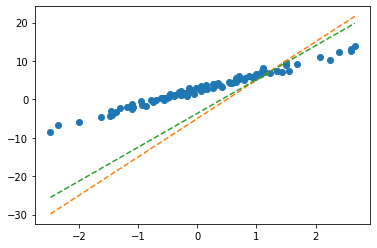

Stage3: Learn (=estimate $\bf\hat{W})$

- 이 과정은 Stage1,2를 반복하면 된다.

What= torch.tensor([-5.0,10.0],requires_grad=True) #

alpha=0.001 
for epoc in range(30): ## 30번 반복합니다!! 
    yhat=X@What 
    loss=torch.sum((y-yhat)**2)
    loss.backward() 
    What.data = What.data-alpha * What.grad
    What.grad=None

원래 철자는 epoch이 맞아요

- 반복결과는?! (최종적으로 구해지는 What의 값은?!) - 참고로 true

What.data ## true인 (2.5,4)와 상당히 비슷함

tensor([2.4290, 4.0144])

- 반복결과를 시각화하면?

plt.plot(x,y,'o')
plt.plot(x,X@What.data,'--')

파라메터의 학습과정 음미 (학습과정 모니터링)

학습과정의 기록

- 기록을 해보자.

loss_history = [] # 기록하고 싶은것 1  
yhat_history = [] # 기록하고 싶은것 2 
What_history = [] # 기록하고 싶은것 3

What= torch.tensor([-5.0,10.0],requires_grad=True)
alpha=0.001 
for epoc in range(30): 
    yhat=X@What ; yhat_history.append(yhat.data.tolist())
    loss=torch.sum((y-yhat)**2); loss_history.append(loss.item())
    loss.backward() 
    What.data = What.data-alpha * What.grad; What_history.append(What.data.tolist())
    What.grad=None

- $\hat{y}$ 관찰 (epoch=3, epoch=10, epoch=15)

plt.plot(x,y,'o')
plt.plot(x,yhat_history[2],'--')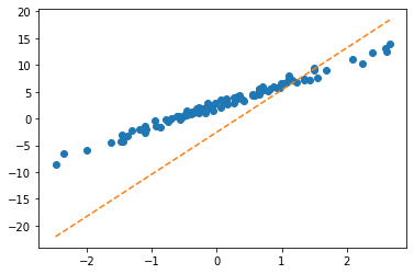

plt.plot(x,y,'o')
plt.plot(x,yhat_history[9],'--')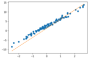

plt.plot(x,y,'o')
plt.plot(x,yhat_history[14],'--')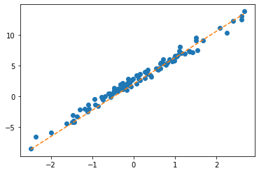

- $\hat{\bf W}$ 관찰

What_history

[[-3.657747745513916, 8.81106948852539],
 [-2.554811716079712, 7.861191749572754],
 [-1.649186372756958, 7.101552963256836],
 [-0.9060714244842529, 6.49347448348999],
 [-0.29667872190475464, 6.006272315979004],
 [0.2027742564678192, 5.615575313568115],
 [0.6119104623794556, 5.302003860473633],
 [0.9469034075737, 5.0501298904418945],
 [1.2210698127746582, 4.847658157348633],
 [1.4453644752502441, 4.684779644012451],
 [1.6287914514541626, 4.553659915924072],
 [1.7787461280822754, 4.448036193847656],
 [1.9012980461120605, 4.3628973960876465],
 [2.0014259815216064, 4.294229507446289],
 [2.0832109451293945, 4.238814353942871],
 [2.149996757507324, 4.194070339202881],
 [2.204521894454956, 4.157923698425293],
 [2.249027729034424, 4.128708839416504],
 [2.285348415374756, 4.105085849761963],
 [2.31498384475708, 4.0859761238098145],
 [2.339160442352295, 4.070511341094971],
 [2.3588807582855225, 4.057991027832031],
 [2.3749637603759766, 4.0478515625],
 [2.3880786895751953, 4.039637088775635],
 [2.3987717628479004, 4.032979965209961],
 [2.40748929977417, 4.027583599090576],
 [2.414595603942871, 4.023208141326904],
 [2.4203879833221436, 4.019659042358398],
 [2.4251089096069336, 4.016779899597168],
 [2.4289560317993164, 4.014443874359131]]

- loss 관찰

plt.plot(loss_history)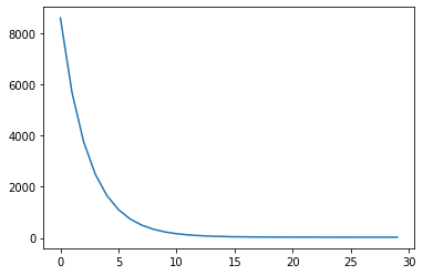

학습과정을 animation으로 시각화

from matplotlib import animation

plt.rcParams['figure.figsize'] = (7.5,2.5)
plt.rcParams["animation.html"] = "jshtml"

- 왼쪽에는 $(x_i,y_i)$ and $(x_i,\hat{y}_i)$ 을 그리고 오른쪽에는 $loss(w_0,w_1)$ 을 그릴것임

fig = plt.figure()
ax1 = fig.add_subplot(1, 2, 1)
ax2 = fig.add_subplot(1, 2, 2, projection='3d')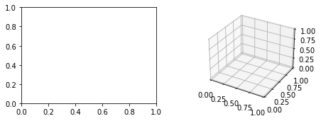

- 왼쪽그림!

ax1.plot(x,y,'o')
line, = ax1.plot(x,yhat_history[0]) # 나중에 애니메이션 할때 필요해요..

fig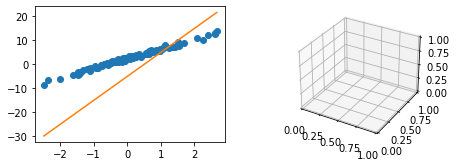

- 오른쪽 그림1: $loss(w_0,w_1)$

_w0 = np.arange(-6, 11, 0.5) ## 파란색곡면을 그리는 코드 (시작) 
_w1 = np.arange(-6, 11, 0.5)
w1,w0 = np.meshgrid(_w1,_w0)
lss=w0*0
for i in range(len(_w0)):
    for j in range(len(_w1)):
        lss[i,j]=torch.sum((y-_w0[i]-_w1[j]*x)**2)
ax2.plot_surface(w0, w1, lss, rstride=1, cstride=1, color='b',alpha=0.35) ## 파란색곡면을 그리는 코드(끝) 
ax2.azim = 40  ## 3d plot의 view 조절 
ax2.dist = 8   ## 3d plot의 view 조절 
ax2.elev = 5   ## 3d plot의 view 조절

fig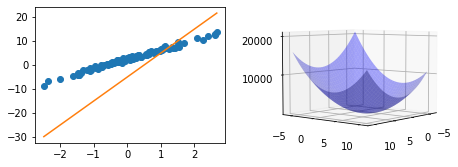

- 오른쪽 그림2: $(w_0,w_1)=(2.5,4)$ 와 $loss(2.5,4)$ 값 <- loss 함수가 최소가 되는 값 (이거 진짜야? ㅋㅋ)

ax2.scatter(2.5,4,torch.sum((y-2.5-4*x)**2),s=200,color='red',marker='*') ## 최소점을 표시하는 코드 (붉은색 별)

<mpl_toolkits.mplot3d.art3d.Path3DCollection at 0x7ffa9199ce90>

fig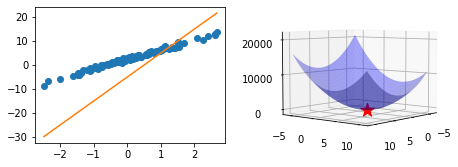

- 오른쪽 그림3: $(w_0,w_1)=(-3.66, 8.81)$ 와 $loss(-3.66,8.81)$ 값

What_history[0]

[-3.657747745513916, 8.81106948852539]

ax2.scatter(What_history[0][0],What_history[0][1],loss_history[0],color='grey') ## 업데이트되는 What을 표시하는 점 (파란색 동그라미)

<mpl_toolkits.mplot3d.art3d.Path3DCollection at 0x7ffa78c2ba10>

fig

- 애니메이션

def animate(epoc):
    line.set_ydata(yhat_history[epoc])
    ax2.scatter(What_history[epoc][0],What_history[epoc][1],loss_history[epoc],color='grey')
    return line

ani = animation.FuncAnimation(fig, animate, frames=30)
plt.close()
ani

- 함수로 만들자..

def show_lrpr(data,history):
    x,y = data 
    loss_history,yhat_history,What_history = history 
    
    fig = plt.figure()
    ax1 = fig.add_subplot(1, 2, 1)
    ax2 = fig.add_subplot(1, 2, 2, projection='3d')

    ## ax1: 왼쪽그림 
    ax1.plot(x,y,'o')
    line, = ax1.plot(x,yhat_history[0]) 
    ## ax2: 오른쪽그림 
    _w0 = np.arange(-6, 11, 0.5) ## 파란색곡면을 그리는 코드 (시작) 
    _w1 = np.arange(-6, 11, 0.5)
    w1,w0 = np.meshgrid(_w1,_w0)
    lss=w0*0
    for i in range(len(_w0)):
        for j in range(len(_w1)):
            lss[i,j]=torch.sum((y-_w0[i]-_w1[j]*x)**2)
    ax2.plot_surface(w0, w1, lss, rstride=1, cstride=1, color='b',alpha=0.35) ## 파란색곡면을 그리는 코드(끝) 
    ax2.scatter(2.5,4,torch.sum((y-2.5-4*x)**2),s=200,color='red',marker='*') ## 최소점을 표시하는 코드 (붉은색 별) 
    ax2.scatter(What_history[0][0],What_history[0][1],loss_history[0],color='b') ## 업데이트되는 What을 표시하는 점 (파란색 동그라미) 
    ax2.azim = 40  ## 3d plot의 view 조절 
    ax2.dist = 8   ## 3d plot의 view 조절 
    ax2.elev = 5   ## 3d plot의 view 조절 

    def animate(epoc):
        line.set_ydata(yhat_history[epoc])
        ax2.scatter(np.array(What_history)[epoc,0],np.array(What_history)[epoc,1],loss_history[epoc],color='grey')
        return line

    ani = animation.FuncAnimation(fig, animate, frames=30)
    plt.close()
    return ani

show_lrpr([x,y],[loss_history,yhat_history,What_history])

$\alpha$에 대하여 ($\alpha$는 학습률)

(1) $\alpha=0.0001$: $\alpha$ 가 너무 작다면? $\to$ 비효율적이다.

loss_history = [] # 기록하고 싶은것 1  
yhat_history = [] # 기록하고 싶은것 2 
What_history = [] # 기록하고 싶은것 3

What= torch.tensor([-5.0,10.0],requires_grad=True)
alpha=0.0001 
for epoc in range(30): 
    yhat=X@What ; yhat_history.append(yhat.data.tolist())
    loss=torch.sum((y-yhat)**2); loss_history.append(loss.item())
    loss.backward() 
    What.data = What.data-alpha * What.grad; What_history.append(What.data.tolist())
    What.grad=None

show_lrpr([x,y],[loss_history,yhat_history,What_history])

(2) $\alpha=0.0083$: $\alpha$가 너무 크다면? $\to$ 다른의미에서 비효율적이다 + 위험하다..

loss_history = [] # 기록하고 싶은것 1  
yhat_history = [] # 기록하고 싶은것 2 
What_history = [] # 기록하고 싶은것 3

What= torch.tensor([-5.0,10.0],requires_grad=True)
alpha=0.0083
for epoc in range(30): 
    yhat=X@What ; yhat_history.append(yhat.data.tolist())
    loss=torch.sum((y-yhat)**2); loss_history.append(loss.item())
    loss.backward() 
    What.data = What.data-alpha * What.grad; What_history.append(What.data.tolist())
    What.grad=None

show_lrpr([x,y],[loss_history,yhat_history,What_history])

(3) $\alpha=0.0085$

loss_history = [] # 기록하고 싶은것 1  
yhat_history = [] # 기록하고 싶은것 2 
What_history = [] # 기록하고 싶은것 3

What= torch.tensor([-5.0,10.0],requires_grad=True)
alpha=0.0085
for epoc in range(30): 
    yhat=X@What ; yhat_history.append(yhat.data.tolist())
    loss=torch.sum((y-yhat)**2); loss_history.append(loss.item())
    loss.backward() 
    What.data = What.data-alpha * What.grad.data; What_history.append(What.data.tolist())
    What.grad=None

show_lrpr([x,y],[loss_history,yhat_history,What_history])

(4) $\alpha=0.01$

loss_history = [] # 기록하고 싶은것 1  
yhat_history = [] # 기록하고 싶은것 2 
What_history = [] # 기록하고 싶은것 3

What= torch.tensor([-5.0,10.0],requires_grad=True)
alpha=0.01
for epoc in range(30): 
    yhat=X@What ; yhat_history.append(yhat.data.tolist())
    loss=torch.sum((y-yhat)**2); loss_history.append(loss.item())
    loss.backward() 
    What.data = What.data-alpha * What.grad; What_history.append(What.data.tolist())
    What.grad=None

show_lrpr([x,y],[loss_history,yhat_history,What_history])

숙제

- 학습률($\alpha$)를 조정하며 실습해보고 스크린샷 제출

03wk-2: 딥러닝의 기초 (1)

강의영상

imports

로드맵

ref

회귀모형 소개

회귀모형에서 데이터 생성

회귀모형에서 학습이란?

파라메터를 학습하는 방법 (적당한 선으로 업데이트 하는 방법)

Stage1: 첫번째 점선 – 임의의 선을 일단 그어보자

Stage2: 첫번째 수정 – 최초의 점선에 대한 ‘적당한 정도’를 판단하고 더 ’적당한’ 점선으로 업데이트 한다.

`#` Stage2를 위한 경사하강법 복습

Stage3: Learn (=estimate \(\bf\hat{W})\)

파라메터의 학습과정 음미 (학습과정 모니터링)

학습과정의 기록

학습과정을 animation으로 시각화

\(\alpha\)에 대하여 (\(\alpha\)는 학습률)

(1) \(\alpha=0.0001\): \(\alpha\) 가 너무 작다면? \(\to\) 비효율적이다.

(2) \(\alpha=0.0083\): \(\alpha\)가 너무 크다면? \(\to\) 다른의미에서 비효율적이다 + 위험하다..

(3) \(\alpha=0.0085\)

(4) \(\alpha=0.01\)

숙제

강의영상

imports

로드맵

ref

회귀모형 소개

회귀모형에서 데이터 생성

회귀모형에서 학습이란?

파라메터를 학습하는 방법 (적당한 선으로 업데이트 하는 방법)

Stage1: 첫번째 점선 – 임의의 선을 일단 그어보자

Stage2: 첫번째 수정 – 최초의 점선에 대한 ‘적당한 정도’를 판단하고 더 ’적당한’ 점선으로 업데이트 한다.

# Stage2를 위한 경사하강법 복습

Stage3: Learn (=estimate \(\bf\hat{W})\)

파라메터의 학습과정 음미 (학습과정 모니터링)

학습과정의 기록

학습과정을 animation으로 시각화

\(\alpha\)에 대하여 (\(\alpha\)는 학습률)

(1) \(\alpha=0.0001\): \(\alpha\) 가 너무 작다면? \(\to\) 비효율적이다.

(2) \(\alpha=0.0083\): \(\alpha\)가 너무 크다면? \(\to\) 다른의미에서 비효율적이다 + 위험하다..

(3) \(\alpha=0.0085\)

(4) \(\alpha=0.01\)

숙제

`#` Stage2를 위한 경사하강법 복습