# !pip install autogluon.multimodal 14wk-58: 전주시기온 / 시계열자료분석
1. 강의영상
2. Imports
import numpy as np
import pandas as pd
import matplotlib.pyplot as plt
#---#
from autogluon.timeseries import TimeSeriesDataFrame, TimeSeriesPredictor
#---#
import os
import warnings
warnings.filterwarnings('ignore')
3. Data
df = pd.read_csv('https://raw.githubusercontent.com/guebin/DV2022/master/posts/temp.csv').iloc[:,2:4].set_axis(['date','temp'],axis=1).assign(date= lambda df: df.date.apply(pd.to_datetime))
df_train = df[:580].assign(item_id = '평균기온')
df_test = df[580:].assign(item_id = '평균기온')
display(df_train.head())
display(df_test.head())| date | temp | item_id | |
|---|---|---|---|
| 0 | 2020-01-01 | -0.5 | 평균기온 |
| 1 | 2020-01-02 | 1.4 | 평균기온 |
| 2 | 2020-01-03 | 2.6 | 평균기온 |
| 3 | 2020-01-04 | 2.0 | 평균기온 |
| 4 | 2020-01-05 | 2.5 | 평균기온 |
| date | temp | item_id | |
|---|---|---|---|
| 580 | 2021-08-03 | 27.5 | 평균기온 |
| 581 | 2021-08-04 | 28.7 | 평균기온 |
| 582 | 2021-08-05 | 28.6 | 평균기온 |
| 583 | 2021-08-06 | 28.1 | 평균기온 |
| 584 | 2021-08-07 | 27.6 | 평균기온 |
여기에서 세번째 칼럼은 오토글루온으로 시계열을 적합하기 위한 인덱스 역할을 함.
plt.plot(df_train.date,df_train.temp)
plt.plot(df_test.date,df_test.temp)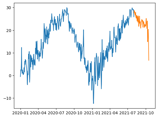
- Tabular 형태의 자료분석이 맵핑 “X -> y” 를 배우는 것이라면, 시계열(timeseries)형태의 자료분석은 맵핑 “y과거 -> y미래” 를 배우는 것이다.
4. 시계열분석의 이해
- 개요: 오토글루온에서 tabular 자료의 분석과 timeseries 분석을 비교하면?
- Tabular:
predictr.fit(df_trian)/predictr.predict(df_test) - TimeSeries:
predictr.fit(ts_train)/predictr.predict(ts_train)
실제로 시계열자료에서
df_test는 주어지지 않음.
- 오토글루온에서 분석가능한 시계열 자료의 형태
1. 하나의 시계열
df1 = pd.DataFrame({'시간':['2023-12-07','2023-12-08'], '종목':['삼성전자']*2, '주가':[72600, 72800]})
df1| 시간 | 종목 | 주가 | |
|---|---|---|---|
| 0 | 2023-12-07 | 삼성전자 | 72600 |
| 1 | 2023-12-08 | 삼성전자 | 72800 |
ts1 = TimeSeriesDataFrame(
    data = df1,
    static_features = None,
    id_column = '종목',
    timestamp_column = '시간'
)
ts1| 주가 | ||
|---|---|---|
| item_id | timestamp | |
| 삼성전자 | 2023-12-07 | 72600 |
| 2023-12-08 | 72800 |
2. 여러개의 시계열
df2 = pd.DataFrame({'시간':['2023-12-07','2023-12-08']*2, '종목':['삼성전자']*2+['카카오']*2, '주가':[72600, 72800, 51700, 51600]})
df2| 시간 | 종목 | 주가 | |
|---|---|---|---|
| 0 | 2023-12-07 | 삼성전자 | 72600 |
| 1 | 2023-12-08 | 삼성전자 | 72800 |
| 2 | 2023-12-07 | 카카오 | 51700 |
| 3 | 2023-12-08 | 카카오 | 51600 |
ts2 = TimeSeriesDataFrame(
    data = df2,
    static_features = None,
    id_column = '종목',
    timestamp_column = '시간'
)
ts2| 주가 | ||
|---|---|---|
| item_id | timestamp | |
| 삼성전자 | 2023-12-07 | 72600 |
| 2023-12-08 | 72800 | |
| 카카오 | 2023-12-07 | 51700 |
| 2023-12-08 | 51600 |
3. 여러개의 시계열 + static_feature
df2 = pd.DataFrame({'시간':['2023-12-07','2023-12-08']*2, '종목':['삼성전자']*2+['카카오']*2, '주가':[72600, 72800, 51700, 51600]})
df3 = pd.DataFrame({'종목':['삼성전자','카카오'],'특징1(기업성격)':['제조','IT'],'특징2(사원수)':[500,25]})
display(df2,df3)
#---#
ts23 = TimeSeriesDataFrame(
    data = df2,
    static_features = df3,
    id_column = '종목',
    timestamp_column = '시간'
)
ts23| 시간 | 종목 | 주가 | |
|---|---|---|---|
| 0 | 2023-12-07 | 삼성전자 | 72600 |
| 1 | 2023-12-08 | 삼성전자 | 72800 |
| 2 | 2023-12-07 | 카카오 | 51700 |
| 3 | 2023-12-08 | 카카오 | 51600 |
| 종목 | 특징1(기업성격) | 특징2(사원수) | |
|---|---|---|---|
| 0 | 삼성전자 | 제조 | 500 |
| 1 | 카카오 | IT | 25 |
| 주가 | ||
|---|---|---|
| item_id | timestamp | |
| 삼성전자 | 2023-12-07 | 72600 |
| 2023-12-08 | 72800 | |
| 카카오 | 2023-12-07 | 51700 |
| 2023-12-08 | 51600 |
5. 적합
A. Step1: 데이터의 정리
ts_train = TimeSeriesDataFrame(
    data = df_train,
    static_features = None,
    id_column = 'item_id',
    timestamp_column = 'date'
)
B. Step2: TimeSeriesPredictor 생성
predictr = TimeSeriesPredictor(
    target = 'temp', # 예측하고 싶은것
    known_covariates_names = None, # 온도를 예측할때 쓸 수 있는 다른 시계열 자료
    prediction_length = len(df_test), # 예측하고 싶은 자료의 길이
    freq = 'D' # 주기 (보통은 'D', 'H'를 씀, 일반적으로 명시하지 않아도 오토글루온이 알아서 찾아줌)
)
C. Step3: 학습
predictr.fit(ts_train,presets='medium_quality')Beginning AutoGluon training...
AutoGluon will save models to 'AutogluonModels/ag-20231209_020312'
=================== System Info ===================
AutoGluon Version: 1.0.0
Python Version: 3.11.6
Operating System: Linux
Platform Machine: x86_64
Platform Version: #140-Ubuntu SMP Thu Aug 4 02:23:37 UTC 2022
CPU Count: 128
GPU Count: 1
Memory Avail: 401.20 GB / 503.74 GB (79.6%)
Disk Space Avail: 1159.47 GB / 1757.88 GB (66.0%)
===================================================
Setting presets to: medium_quality
Fitting with arguments:
{'enable_ensemble': True,
'eval_metric': WQL,
'freq': 'D',
'hyperparameters': 'light',
'known_covariates_names': [],
'num_val_windows': 1,
'prediction_length': 76,
'quantile_levels': [0.1, 0.2, 0.3, 0.4, 0.5, 0.6, 0.7, 0.8, 0.9],
'random_seed': 123,
'refit_every_n_windows': 1,
'refit_full': False,
'target': 'temp',
'verbosity': 2}
Provided train_data has 580 rows, 1 time series. Median time series length is 580 (min=580, max=580).
Provided dataset contains following columns:
target: 'temp'
AutoGluon will gauge predictive performance using evaluation metric: 'WQL'
This metric's sign has been flipped to adhere to being higher_is_better. The metric score can be multiplied by -1 to get the metric value.
===================================================
Starting training. Start time is 2023-12-09 02:03:12
Models that will be trained: ['Naive', 'SeasonalNaive', 'ETS', 'Theta', 'RecursiveTabular', 'DirectTabular', 'TemporalFusionTransformer']
Training timeseries model Naive.
-0.2088 = Validation score (-WQL)
0.00 s = Training runtime
0.99 s = Validation (prediction) runtime
Training timeseries model SeasonalNaive.
-0.1648 = Validation score (-WQL)
0.00 s = Training runtime
0.97 s = Validation (prediction) runtime
Training timeseries model ETS.
-0.2091 = Validation score (-WQL)
0.00 s = Training runtime
14.10 s = Validation (prediction) runtime
Training timeseries model Theta.
-0.2281 = Validation score (-WQL)
0.00 s = Training runtime
16.11 s = Validation (prediction) runtime
Training timeseries model RecursiveTabular.
-0.2031 = Validation score (-WQL)
1.17 s = Training runtime
0.54 s = Validation (prediction) runtime
Training timeseries model DirectTabular.
-0.0976 = Validation score (-WQL)
3.83 s = Training runtime
0.06 s = Validation (prediction) runtime
Training timeseries model TemporalFusionTransformer.
-0.0648 = Validation score (-WQL)
43.09 s = Training runtime
0.02 s = Validation (prediction) runtime
Fitting simple weighted ensemble.
Ensemble weights: {'RecursiveTabular': 0.03, 'TemporalFusionTransformer': 0.97}
-0.0644 = Validation score (-WQL)
0.54 s = Training runtime
0.56 s = Validation (prediction) runtime
Training complete. Models trained: ['Naive', 'SeasonalNaive', 'ETS', 'Theta', 'RecursiveTabular', 'DirectTabular', 'TemporalFusionTransformer', 'WeightedEnsemble']
Total runtime: 81.49 s
Best model: WeightedEnsemble
Best model score: -0.0644<autogluon.timeseries.predictor.TimeSeriesPredictor at 0x7f1ecc493a10>D. Step4: 예측
predictr.predict(ts_train)Model not specified in predict, will default to the model with the best validation score: WeightedEnsemble| mean | 0.1 | 0.2 | 0.3 | 0.4 | 0.5 | 0.6 | 0.7 | 0.8 | 0.9 | ||
|---|---|---|---|---|---|---|---|---|---|---|---|
| item_id | timestamp | ||||||||||
| 평균기온 | 2021-08-03 | 28.914501 | 24.795792 | 26.168787 | 27.809203 | 29.570845 | 28.914501 | 29.099419 | 30.381727 | 31.509549 | 32.979891 |
| 2021-08-04 | 29.011972 | 25.224210 | 26.569047 | 27.891114 | 29.409711 | 29.011973 | 29.539519 | 30.630746 | 31.646940 | 32.617147 | |
| 2021-08-05 | 28.963903 | 25.303622 | 26.652311 | 27.791000 | 28.911906 | 28.963904 | 29.627844 | 30.573073 | 31.487950 | 32.178999 | |
| 2021-08-06 | 28.879606 | 25.321959 | 26.679040 | 27.704727 | 28.464277 | 28.879606 | 29.533904 | 30.426272 | 31.194846 | 31.836305 | |
| 2021-08-07 | 28.848444 | 25.428517 | 26.768485 | 27.721187 | 28.241648 | 28.848443 | 29.432855 | 30.302661 | 30.940070 | 31.615334 | |
| ... | ... | ... | ... | ... | ... | ... | ... | ... | ... | ... | |
| 2021-10-13 | 17.223763 | 14.030822 | 14.937548 | 15.708939 | 16.554551 | 17.223762 | 17.925664 | 18.405870 | 19.422831 | 20.733676 | |
| 2021-10-14 | 16.985195 | 13.724998 | 14.696005 | 15.360775 | 16.284362 | 16.985195 | 17.686742 | 18.160193 | 19.193498 | 20.484604 | |
| 2021-10-15 | 16.801191 | 13.507242 | 14.529965 | 15.083086 | 16.092644 | 16.801192 | 17.514405 | 17.965267 | 19.019064 | 20.290269 | |
| 2021-10-16 | 16.448746 | 13.160046 | 14.224872 | 14.662191 | 15.767436 | 16.448745 | 17.196025 | 17.600139 | 18.683899 | 19.935804 | |
| 2021-10-17 | 15.980749 | 12.734847 | 13.844127 | 14.156934 | 15.373598 | 15.980749 | 16.800518 | 17.121816 | 18.252594 | 19.484188 |
76 rows × 10 columns
E. 시각화
predictions = predictr.predict(ts_train)
predictions
Model not specified in predict, will default to the model with the best validation score: WeightedEnsemble| mean | 0.1 | 0.2 | 0.3 | 0.4 | 0.5 | 0.6 | 0.7 | 0.8 | 0.9 | ||
|---|---|---|---|---|---|---|---|---|---|---|---|
| item_id | timestamp | ||||||||||
| 평균기온 | 2021-08-03 | 28.914501 | 24.795792 | 26.168787 | 27.809203 | 29.570845 | 28.914501 | 29.099419 | 30.381727 | 31.509549 | 32.979891 |
| 2021-08-04 | 29.011972 | 25.224210 | 26.569047 | 27.891114 | 29.409711 | 29.011973 | 29.539519 | 30.630746 | 31.646940 | 32.617147 | |
| 2021-08-05 | 28.963903 | 25.303622 | 26.652311 | 27.791000 | 28.911906 | 28.963904 | 29.627844 | 30.573073 | 31.487950 | 32.178999 | |
| 2021-08-06 | 28.879606 | 25.321959 | 26.679040 | 27.704727 | 28.464277 | 28.879606 | 29.533904 | 30.426272 | 31.194846 | 31.836305 | |
| 2021-08-07 | 28.848444 | 25.428517 | 26.768485 | 27.721187 | 28.241648 | 28.848443 | 29.432855 | 30.302661 | 30.940070 | 31.615334 | |
| ... | ... | ... | ... | ... | ... | ... | ... | ... | ... | ... | |
| 2021-10-13 | 17.223763 | 14.030822 | 14.937548 | 15.708939 | 16.554551 | 17.223762 | 17.925664 | 18.405870 | 19.422831 | 20.733676 | |
| 2021-10-14 | 16.985195 | 13.724998 | 14.696005 | 15.360775 | 16.284362 | 16.985195 | 17.686742 | 18.160193 | 19.193498 | 20.484604 | |
| 2021-10-15 | 16.801191 | 13.507242 | 14.529965 | 15.083086 | 16.092644 | 16.801192 | 17.514405 | 17.965267 | 19.019064 | 20.290269 | |
| 2021-10-16 | 16.448746 | 13.160046 | 14.224872 | 14.662191 | 15.767436 | 16.448745 | 17.196025 | 17.600139 | 18.683899 | 19.935804 | |
| 2021-10-17 | 15.980749 | 12.734847 | 13.844127 | 14.156934 | 15.373598 | 15.980749 | 16.800518 | 17.121816 | 18.252594 | 19.484188 |
76 rows × 10 columns
plt.plot(df_train.date,df_train.temp,label='observed')
plt.plot(df_test.date,df_test.temp,color='gray',alpha=0.5,label='future value')
plt.plot(df_test.date,predictions['mean'],color='C1',label='estimated')
plt.fill_between(df_test.date, predictions['0.1'], predictions['0.9'],color='C1',alpha=0.2)
plt.legend()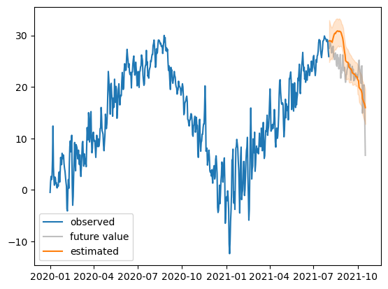
- 이정도 결과는 합리적으로 보임
5. 연구 및 토의
A. static_feature vs known_covariates
- static은 시점에 따라 변화하지 않는 정보, known_covariates는 시점에 따라 변화하지만 이미 알고있는 미래시계열
- 분석타입1: fit(target의 현재까지자료) / forecast(target의 현재까지자료) = target의 미래
- 분석타입2: fit(target의 현재까지자료,static_feature) -> forecast(target의 현재까지자료,static_feature) = target의 미래
- 분석타입3: fit(target의 현재까지자료,known_covariates의 현재까지자료) -> forecast(target의 현재까지자료,known_covariates의 미래) = target의 미래
B. 장기예측
df = pd.read_csv('https://raw.githubusercontent.com/guebin/DV2022/master/posts/temp.csv').iloc[:,2:4].set_axis(['date','temp'],axis=1).assign(date= lambda df: df.date.apply(pd.to_datetime))
df_train = df[:513].assign(item_id = '평균기온')
df_test = df[513:].assign(item_id = '평균기온')
#---#
## step1
ts_train = TimeSeriesDataFrame(
    data = df_train,
    static_features = None,
    id_column = 'item_id',
    timestamp_column = 'date'
)
## step2
predictr = TimeSeriesPredictor(
    target = 'temp', # 예측하고 싶은것
    known_covariates_names = None, # 온도를 예측할때 쓸 수 있는 다른 시계열 자료
    prediction_length = len(df_test), # 예측하고 싶은 자료의 길이
    freq = 'D' # 주기 (보통은 'D', 'H'를 씀, 일반적으로 명시하지 않아도 오토글루온이 알아서 찾아줌)
)
## step3
predictr.fit(ts_train)
## step4
predictr.predict(ts_train)
#---#
predictions = predictr.predict(ts_train)
plt.plot(df_train.date,df_train.temp,label='observed')
plt.plot(df_test.date,df_test.temp,color='gray',alpha=0.5,label='future value')
plt.plot(df_test.date,predictions['mean'],color='C1',label='estimated')
plt.fill_between(df_test.date, predictions['0.1'], predictions['0.9'],color='C1',alpha=0.2)
plt.legend()
No path specified. Models will be saved in: "AutogluonModels/ag-20231209_020014"
Beginning AutoGluon training...
AutoGluon will save models to 'AutogluonModels/ag-20231209_020014'
=================== System Info ===================
AutoGluon Version: 1.0.0
Python Version: 3.11.6
Operating System: Linux
Platform Machine: x86_64
Platform Version: #140-Ubuntu SMP Thu Aug 4 02:23:37 UTC 2022
CPU Count: 128
GPU Count: 1
Memory Avail: 403.68 GB / 503.74 GB (80.1%)
Disk Space Avail: 1159.48 GB / 1757.88 GB (66.0%)
===================================================
Fitting with arguments:
{'enable_ensemble': True,
'eval_metric': WQL,
'freq': 'D',
'hyperparameters': 'default',
'known_covariates_names': [],
'num_val_windows': 1,
'prediction_length': 143,
'quantile_levels': [0.1, 0.2, 0.3, 0.4, 0.5, 0.6, 0.7, 0.8, 0.9],
'random_seed': 123,
'refit_every_n_windows': 1,
'refit_full': False,
'target': 'temp',
'verbosity': 2}
Provided train_data has 513 rows, 1 time series. Median time series length is 513 (min=513, max=513).
Provided dataset contains following columns:
target: 'temp'
AutoGluon will gauge predictive performance using evaluation metric: 'WQL'
This metric's sign has been flipped to adhere to being higher_is_better. The metric score can be multiplied by -1 to get the metric value.
===================================================
Starting training. Start time is 2023-12-09 02:00:14
Models that will be trained: ['SeasonalNaive', 'CrostonSBA', 'NPTS', 'AutoETS', 'DynamicOptimizedTheta', 'AutoARIMA', 'RecursiveTabular', 'DirectTabular', 'DeepAR', 'TemporalFusionTransformer', 'PatchTST']
Training timeseries model SeasonalNaive.
-0.8225 = Validation score (-WQL)
0.00 s = Training runtime
5.26 s = Validation (prediction) runtime
Training timeseries model CrostonSBA.
-0.5749 = Validation score (-WQL)
0.00 s = Training runtime
5.96 s = Validation (prediction) runtime
Training timeseries model NPTS.
-0.5393 = Validation score (-WQL)
0.00 s = Training runtime
1.33 s = Validation (prediction) runtime
Training timeseries model AutoETS.
-0.7227 = Validation score (-WQL)
0.00 s = Training runtime
14.14 s = Validation (prediction) runtime
Training timeseries model DynamicOptimizedTheta.
-0.7426 = Validation score (-WQL)
0.00 s = Training runtime
16.03 s = Validation (prediction) runtime
Training timeseries model AutoARIMA.
-0.7599 = Validation score (-WQL)
0.00 s = Training runtime
9.52 s = Validation (prediction) runtime
Training timeseries model RecursiveTabular.
-0.8312 = Validation score (-WQL)
1.45 s = Training runtime
0.76 s = Validation (prediction) runtime
Training timeseries model DirectTabular.
-0.4099 = Validation score (-WQL)
1.56 s = Training runtime
0.06 s = Validation (prediction) runtime
Training timeseries model DeepAR.
-0.4404 = Validation score (-WQL)
21.42 s = Training runtime
0.44 s = Validation (prediction) runtime
Training timeseries model TemporalFusionTransformer.
-1.9696 = Validation score (-WQL)
36.18 s = Training runtime
0.03 s = Validation (prediction) runtime
Training timeseries model PatchTST.
-0.4265 = Validation score (-WQL)
11.90 s = Training runtime
0.02 s = Validation (prediction) runtime
Fitting simple weighted ensemble.
Ensemble weights: {'DeepAR': 0.26, 'DirectTabular': 0.18, 'PatchTST': 0.52, 'TemporalFusionTransformer': 0.04}
-0.3698 = Validation score (-WQL)
0.82 s = Training runtime
0.55 s = Validation (prediction) runtime
Training complete. Models trained: ['SeasonalNaive', 'CrostonSBA', 'NPTS', 'AutoETS', 'DynamicOptimizedTheta', 'AutoARIMA', 'RecursiveTabular', 'DirectTabular', 'DeepAR', 'TemporalFusionTransformer', 'PatchTST', 'WeightedEnsemble']
Total runtime: 126.97 s
Best model: WeightedEnsemble
Best model score: -0.3698
Model not specified in predict, will default to the model with the best validation score: WeightedEnsemble
Model not specified in predict, will default to the model with the best validation score: WeightedEnsemble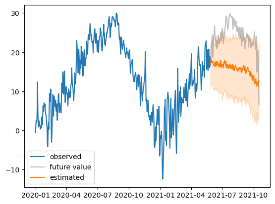
- 장기예측은 그럴듯하지 않아보임 – 장기예측은 (좁은의미의)시계열분석의 범위를 벗어남
- 통계학과에서 배우는 시계열분석
- 주식시계열: 독립인듯 하지만, 사실은 독립이 아닌자료. 즉 “관측자료 = 정보 + 오차” 인데, 오차항이 독립이 아닐 경우.
- 오차항이 독립이 아니라는 의미: 주식시계열이 비합리적인 관측자료라는 의미임. (사실 오차항은 독립이어야 하지 않냐?)
- 주식시계열자료의 새로운해석: 원래 우리가 통계에서 다루는 셋팅은 “관측자료 = 정보 + 오차”이다.1. 이를 시계열로 바꿔서 표현하면 “주식시계열자료 = 합리적정보 + 오차 = 합리적정보 + (기세 + 독립오차)”
- 시계열분석: 통계학과에서 배우는 시계열모형들은 “기세”를 모델링하는 것임. 즉 비합리적인 오차항을 모델링 하는 것!
- 1시점 전의 기세의 영향을 얼만큼 강하게 볼지 결정하는 일은, AR(1)의 계수값을 결정하는 일과 같은 일이다.
- 몇 시점까지의 기세를 봐야할지 결정하는 일은 AR(p)모형에서 p의 값을 결정하는 일과 같은 일이다.
- 100시점 전까지의 기세를 보고싶다면, 원칙적으로는 AR(100)을 적합해야하지만 그렇다면 너무 학습할 파라메터가 많을 것임. 하지만 이론에 따라서 AR(100)과 비슷한 효과를 주고 파라메터를 더 적게 가지는 MA(q), ARMA(p,q) 와 같은 모형이 존재함이 밝혀짐. 그래서 아주 먼 시점의 기세까지 파악하여 분석해야 한다면 ARMA(p,q)를 적합하는 것이 유리함.
- 트렌드와 계절성을 가지는 시계열 자료는 기세를 모델링하기 어려운데 어쩌지? 제거하고 분석 (ARIMA, SARIMA 등의 개발)
- 기세의 변동성이 시간에 따라 달라진다면 어쩌지? ARCH, GARCH 의 개발
- 평균정보: 시계열분석에서 합리적정보(평균정보)는
static_feature,known_covariates에 포함되어있다. - 장기예측: 장기예측은 평균정보를 잘 추정하는것이 중요하며, 이는 기세를 모델링하는 것과는 별 상관이 없다. (즉 “좁은”의미의 시계열분석과 상관이 없다)
- 파업선언: 시계열로 장기예측을 해라? 저는 그냥 다른 방법을 썼어요..
1 참고로 기존에 우리가 다루었던 자료는 엄밀하게 쓰면 “관측자료 = 정보 + 독립오차” 임