import numpy as np
import pandas as pd
import matplotlib.pyplot as plt
import sklearn.tree
import sklearn.ensemble
#---#
import warnings
warnings.filterwarnings('ignore')
#---#
import matplotlib.animation
import IPython12wk-45: 아이스크림 / 부스팅
1. 강의영상
2. Imports
3. Data
np.random.seed(43052)
temp = pd.read_csv('https://raw.githubusercontent.com/guebin/DV2022/master/posts/temp.csv').iloc[:,3].to_numpy()[:80]
temp.sort()
eps = np.random.randn(80)*3 # 오차
icecream_sales = 20 + temp * 2.5 + eps
df_train = pd.DataFrame({'temp':temp,'sales':icecream_sales})
df_train| temp | sales | |
|---|---|---|
| 0 | -4.1 | 10.900261 |
| 1 | -3.7 | 14.002524 |
| 2 | -3.0 | 15.928335 |
| 3 | -1.3 | 17.673681 |
| 4 | -0.5 | 19.463362 |
| ... | ... | ... |
| 75 | 9.7 | 50.813741 |
| 76 | 10.3 | 42.304739 |
| 77 | 10.6 | 45.662019 |
| 78 | 12.1 | 48.739157 |
| 79 | 12.4 | 46.007937 |
80 rows × 2 columns
4. 적합
# step1
X = df_train[['temp']]
y = df_train['sales']
# step2
predictr = sklearn.ensemble.GradientBoostingRegressor()
# step3
predictr.fit(X,y)
# step4
yhat = predictr.predict(X) plt.plot(X,y,'o')
plt.plot(X,yhat,'--')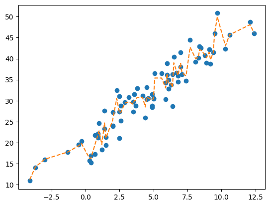
5. yhat을 얻는과정 – 어려움..
- my_trees 생성
trees = [t[0] for t in predictr.estimators_]
trees[0]DecisionTreeRegressor(criterion='friedman_mse', max_depth=3,
random_state=RandomState(MT19937) at 0x7F5A701BB440)In a Jupyter environment, please rerun this cell to show the HTML representation or trust the notebook. On GitHub, the HTML representation is unable to render, please try loading this page with nbviewer.org.
DecisionTreeRegressor(criterion='friedman_mse', max_depth=3,
random_state=RandomState(MT19937) at 0x7F5A701BB440)- 단순시도 (나무들의 평균으로) – 실패
_yhat = np.stack([tree.predict(X) for tree in trees]).mean(axis=0)
_yhatarray([-1.98529568, -1.68873716, -1.50105449, -1.32748757, -1.17877814,
-1.12461928, -1.48130074, -1.47726246, -1.47726246, -1.14576839,
-1.14576839, -0.93324255, -0.93324255, -0.82550938, -1.14740524,
-0.63621774, -0.63621774, -0.99552612, -0.99552612, -0.56894418,
-0.56894418, -0.56894418, -0.05104935, -0.39699577, -0.39699577,
-0.39699577, -0.38296042, -0.38296042, -0.16511506, -0.13001062,
-0.18975132, -0.18975132, -0.09772732, -0.09772732, -0.02478889,
-0.02478889, -0.25650094, -0.02421372, -0.02421372, -0.03653755,
-0.08676362, -0.08676362, -0.08676362, -0.05359582, -0.05359582,
0.43424239, 0.43353213, 0.19572773, 0.19572773, 0.54183429,
0.54183429, 0.2947621 , 0.2947621 , 0.2947621 , 0.21585817,
0.21585817, 0.7964528 , 0.59531418, 0.49763334, 0.49763334,
0.78455561, 0.78455561, 0.55907873, 0.48574479, 1.16729012,
0.89795288, 0.92295305, 1.11059435, 1.09672204, 0.98224138,
0.9138514 , 1.05038217, 0.86805699, 1.04227523, 1.49564195,
1.89066912, 1.19912714, 1.46250802, 1.70344969, 1.51603631])plt.plot(X,y,'o')
plt.plot(X,yhat,'--')
plt.plot(X,_yhat+y.mean(),'--')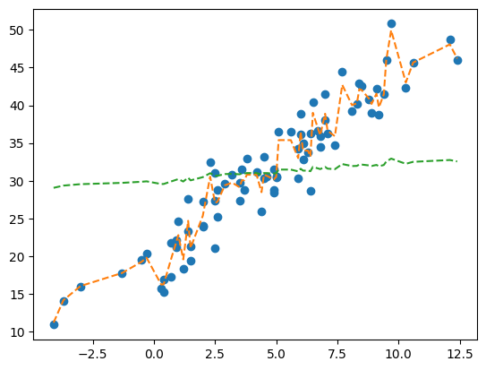
- 처음 3개의 의사결정나무의 예측
plt.plot(X,y,'o')
# plt.plot(X,yhat,'--')
plt.plot(X,trees[0].predict(X)+y.mean(),'--',label='yhat with tree[0]')
plt.plot(X,trees[1].predict(X)+y.mean(),'--',label='yhat with tree[1]')
plt.plot(X,trees[2].predict(X)+y.mean(),'--',label='yhat with tree[2]')
plt.plot(X,trees[-1].predict(X)+y.mean(),'--',label='yhat with tree[-1]')
plt.legend()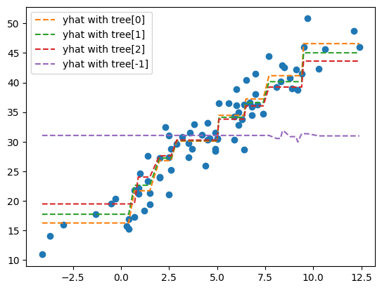
- 비밀이 뭘까?
- 초기값:
yhat=y.mean()으로 적합 – ver 0.0 - 첫번째 나무를 반영하는 방법: 현재까지의 적합값 + 첫번째 나무의 적합값 * 0.1 – ver 0.01
- 두번째 나무를 반영하는 방법: 현재까지의 적합값 + 두번째 나무의 적합값 * 0.1 – ver 0.02
- …
- 100번째 나무를 반영하는 방법: 현재까지의 적합값 + 100번째 나무의 적합값 * 0.1 – ver 1.00
- 시각화로 확인
(trees[0].predict(X)+trees[1].predict(X))array([-28.12857773, -28.12857773, -28.12857773, -28.12857773,
-28.12857773, -28.12857773, -28.12857773, -28.12857773,
-28.12857773, -17.76744106, -17.76744106, -17.76744106,
-17.76744106, -17.76744106, -17.76744106, -17.76744106,
-17.76744106, -17.76744106, -17.76744106, -8.07411483,
-8.07411483, -8.07411483, -8.07411483, -8.07411483,
-8.07411483, -8.07411483, -8.07411483, -8.07411483,
-1.82748008, -1.82748008, -1.82748008, -1.82748008,
-1.82748008, -1.82748008, -1.82748008, -1.82748008,
-1.82748008, -1.82748008, -1.82748008, -1.82748008,
-1.82748008, -1.82748008, -1.82748008, -1.82748008,
-1.82748008, 6.48143774, 6.48143774, 6.48143774,
6.48143774, 6.48143774, 6.48143774, 6.48143774,
6.48143774, 6.48143774, 6.48143774, 6.48143774,
11.74216296, 11.74216296, 11.74216296, 11.74216296,
11.74216296, 11.74216296, 11.74216296, 11.74216296,
19.21655361, 19.21655361, 19.21655361, 19.21655361,
19.21655361, 19.21655361, 19.21655361, 19.21655361,
19.21655361, 19.21655361, 29.52785838, 29.52785838,
29.52785838, 29.52785838, 29.52785838, 29.52785838])predictions = [tree.predict(X) for tree in trees]
plt.plot(X,y,'o',label='RawData')
plt.plot(X,y.mean()+y*0,'--',label='WeakPredictor (ver 0.00)')
plt.plot(
X,
y.mean() + np.stack(predictions[:1]).sum(axis=0)*0.1,
'--',label='WeakPredictor (ver 0.01)'
)
plt.plot(
X,
y.mean() + np.stack(predictions[:2]).sum(axis=0)*0.1 ,
'--',label='WeakPredictor (ver 0.02)'
)
plt.plot(
X,
y.mean() + np.stack(predictions[:3]).sum(axis=0)*0.1,
'--',label='WeakPredictor (ver 0.03)'
)
plt.plot(
X,
y.mean() + np.stack(predictions[:]).sum(axis=0)*0.1,
'--',label='WeakPredictor (ver 1.00)'
)
plt.legend()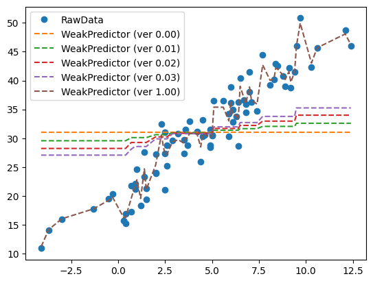
- 애니메이션으로 표현
def ensemble(trees,i=None):
if i is None:
i = len(trees)
else:
i = i+1
yhat = np.stack([tree.predict(X) for tree in trees[:i]]).sum(axis=0)*0.1
return yhat + y.mean()fig = plt.figure()
ax = fig.subplots()
plt.close()
#---#
def func(i):
ax.clear()
ax.plot(X,y,'o',label='RawData')
ax.plot(X,ensemble(trees,i),'--',label=f'WeakPredictor (ver {(i+1)/100:.2f})')
ax.legend()
#---#
ani = matplotlib.animation.FuncAnimation(
fig,func,frames = 50
)
display(IPython.display.HTML(ani.to_jshtml()))6. 재현
trees[0]DecisionTreeRegressor(criterion='friedman_mse', max_depth=3,
random_state=RandomState(MT19937) at 0x7F5A701BB440)In a Jupyter environment, please rerun this cell to show the HTML representation or trust the notebook. On GitHub, the HTML representation is unable to render, please try loading this page with nbviewer.org.
DecisionTreeRegressor(criterion='friedman_mse', max_depth=3,
random_state=RandomState(MT19937) at 0x7F5A701BB440)A. 재현의 확인
- 아이디어:
- 처음부터
yhat을 강하게 학습하지 않고 약하게 조금씩 학습하자. - 부족한 공부는 (=학습이 덜 되어있는 부분 =
y-yhat)은 조금씩 강화하면서 보완하자.
- 구현: my_trees, my_residuals를 직접구현
my_trees = []
my_residuals = [] res = y - y.mean()
# 첫공부
for i in range(100):
tree = sklearn.tree.DecisionTreeRegressor(
criterion = 'friedman_mse',
max_depth=3
)
tree.fit(X,res)
yhat = tree.predict(X)
res = res - yhat * 0.1 # 학습한걸 다 반영하지 말고 0.1정도만 반영. 여기서 0.1은 학습율
my_trees.append(tree)
my_residuals.append(res)- 비교: my_trees와 trees의 비교 (고정된 \(i\))
i=10
fig = plt.figure()
ax = fig.subplots(2,2)
ax[0,0].plot(X,y,'o',alpha=0.5)
ax[0,0].plot(X,ensemble(my_trees,i))
ax[0,1].plot(X,y,'o',alpha=0.5)
ax[0,1].plot(X,ensemble(trees,i))
sklearn.tree.plot_tree(my_trees[i],max_depth=0,ax=ax[1,0]);
sklearn.tree.plot_tree(trees[i],max_depth=0,ax=ax[1,1]);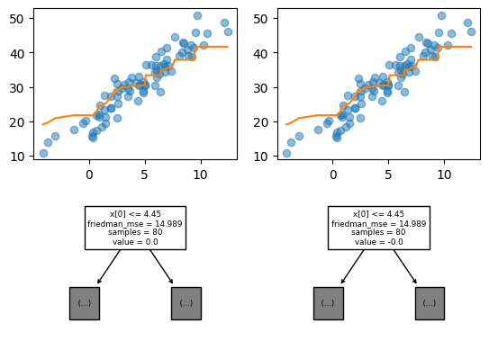
- 비교: my_trees와 trees의 비교 (애니메이션)
#i=10
fig = plt.figure()
ax = fig.subplots(2,2)
plt.close()
#---#
def func(i):
ax[0,0].clear()
ax[0,0].plot(X,y,'o',alpha=0.5)
ax[0,0].plot(X,ensemble(my_trees,i))
#--#
ax[0,1].clear()
ax[0,1].plot(X,y,'o',alpha=0.5)
ax[0,1].plot(X,ensemble(trees,i))
#--#
ax[1,0].clear()
sklearn.tree.plot_tree(my_trees[i],max_depth=0,ax=ax[1,0]);
#--#
ax[1,1].clear()
sklearn.tree.plot_tree(trees[i],max_depth=0,ax=ax[1,1]);
#---#
ani = matplotlib.animation.FuncAnimation(fig,func,frames=100)
display(IPython.display.HTML(ani.to_jshtml()))B. Step별 분석
fig,ax = plt.subplots(1,4,figsize=(8,2))
plt.close()def func(i):
ax[0].clear();
ax[0].plot(X,y,'o',alpha=0.5)
ax[0].plot(X,ensemble(my_trees,i),'--')
ax[0].set_title("Step0")
ax[1].clear();
ax[1].set_ylim(-20,20)
ax[1].plot(X,my_residuals[i],'o',alpha=0.5)
ax[1].set_title("Step1:Residual")
ax[2].clear();
ax[2].set_ylim(-20,20)
ax[2].plot(X,my_residuals[i],'o',alpha=0.5)
ax[2].plot(X,my_trees[i].predict(X),'--')
ax[2].set_title("Step2:Fit")
ax[3].clear();
ax[3].plot(X,y,'o',alpha=0.5)
ax[3].plot(X,ensemble(my_trees,i),'--',color='C1')
ax[3].plot(X,ensemble(my_trees,i+1),'--',color='C3')
ax[3].set_title("Step3:Update") ani = matplotlib.animation.FuncAnimation(
fig,
func,
frames = 50
)display(IPython.display.HTML(ani.to_jshtml()))- 관찰1: “Step1: Residual”은 점점 단순오차차럼 변화한다.
- 관찰2: “Step2: Fit”의 분기점들은 고정된 값이 아니다. (계속 변한다)
- 관찰3: “Step3: Update” 업데이터되는 양은 반복이 진행될수록 점점 작아진다.
- 위의 그림에서
- Step0: 공부할 자료, 현재까지 공부량
- Step1: 남은 공부량
- Step2: 공부! (이해O / 암기X)
- Step3: 공부의 10%의 기억.. 기억나는 것만 두뇌에 update되어있음.
- 느낌: 조금씩 데이터를 학습한다. 학습할 자료가 오차항처럼 보인다면? 그때는 적합을 멈춘다. (오차항을 적합할 필요는 없잖아?)