import numpy as np
import pandas as pd
import matplotlib.pyplot as plt
import sklearn.tree
import sklearn.ensemble
#---#
import warnings
warnings.filterwarnings('ignore')
#---#
import matplotlib.animation
import IPython11wk-43: 아이스크림 판매량 / 배깅
1. 강의영상
2. Imports
3. Data + 의사결정나무로 적합
np.random.seed(43052)
temp = pd.read_csv('https://raw.githubusercontent.com/guebin/DV2022/master/posts/temp.csv').iloc[:,3].to_numpy()[:80]
temp.sort()
eps = np.random.randn(80)*3 # 오차
icecream_sales = 20 + temp * 2.5 + eps
df_train = pd.DataFrame({'temp':temp,'sales':icecream_sales})
df_train| temp | sales | |
|---|---|---|
| 0 | -4.1 | 10.900261 |
| 1 | -3.7 | 14.002524 |
| 2 | -3.0 | 15.928335 |
| 3 | -1.3 | 17.673681 |
| 4 | -0.5 | 19.463362 |
| ... | ... | ... |
| 75 | 9.7 | 50.813741 |
| 76 | 10.3 | 42.304739 |
| 77 | 10.6 | 45.662019 |
| 78 | 12.1 | 48.739157 |
| 79 | 12.4 | 46.007937 |
80 rows × 2 columns
# step1
X = df_train[['temp']]
y = df_train['sales']
# step2
predictr = sklearn.tree.DecisionTreeRegressor()
# step3
predictr.fit(X,y)
# step4 -- passDecisionTreeRegressor()In a Jupyter environment, please rerun this cell to show the HTML representation or trust the notebook.
On GitHub, the HTML representation is unable to render, please try loading this page with nbviewer.org.
DecisionTreeRegressor()
plt.plot(X,y,'o')
plt.plot(X,predictr.predict(X),'--')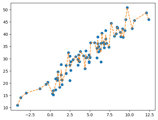
4. 배깅으로 적합
# step1
X = df_train[['temp']]
y = df_train['sales']
# step2
predictr = sklearn.ensemble.BaggingRegressor()
# step3
predictr.fit(X,y)
# step4 -- passBaggingRegressor()In a Jupyter environment, please rerun this cell to show the HTML representation or trust the notebook.
On GitHub, the HTML representation is unable to render, please try loading this page with nbviewer.org.
BaggingRegressor()
plt.plot(X,y,'o')
plt.plot(X,predictr.predict(X),'--')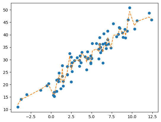
5. 코드뜯어보기
A. 원리
- 알고리즘
- 80개의 샘플에서 80개를 중복을 허용하여 뽑는다.
- 1에서 뽑힌 샘플들을 이용하여 tree를 적합시킨다.
- 1-2를 10번 반복하고 10개의 tree의 평균값을
yhat으로 선택한다.
B. plot_tree 체크
- 10개의 트리들의 리스트
trees = predictr.estimators_
trees
[DecisionTreeRegressor(random_state=1644635363),
DecisionTreeRegressor(random_state=1304269235),
DecisionTreeRegressor(random_state=1794000214),
DecisionTreeRegressor(random_state=1273087880),
DecisionTreeRegressor(random_state=995922005),
DecisionTreeRegressor(random_state=1372517728),
DecisionTreeRegressor(random_state=1087222928),
DecisionTreeRegressor(random_state=3687756),
DecisionTreeRegressor(random_state=1772778467),
DecisionTreeRegressor(random_state=92158766)]- 재표본데이터셋
predictr.estimators_samples_[0] # (X,y)의 쌍을 80개 중복을 허용하여 뽑기 위한 인덱스array([19, 10, 25, 29, 50, 7, 46, 31, 10, 39, 78, 14, 54, 79, 28, 35, 73,
0, 74, 72, 66, 36, 55, 24, 41, 11, 68, 65, 71, 36, 54, 41, 76, 34,
0, 59, 5, 7, 67, 61, 64, 21, 27, 26, 43, 55, 49, 23, 29, 27, 41,
14, 58, 5, 12, 40, 12, 38, 8, 19, 63, 4, 35, 75, 64, 9, 69, 17,
32, 15, 60, 55, 18, 55, 22, 73, 28, 48, 57, 63])samples = predictr.estimators_samples_- 첫번째 트리 재현
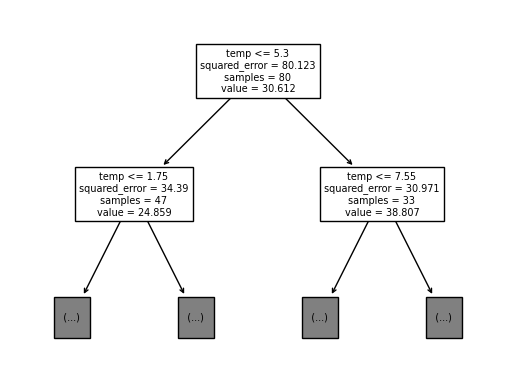
sklearn.tree.plot_tree(
    predictr.estimators_[0],
    feature_names=X.columns,
    max_depth=1
);
X_array = np.array(X)
y_array = np.array(y)
tree = sklearn.tree.DecisionTreeRegressor()
tree.fit(X_array[samples[0]],y_array[samples[0]])DecisionTreeRegressor()In a Jupyter environment, please rerun this cell to show the HTML representation or trust the notebook.
On GitHub, the HTML representation is unable to render, please try loading this page with nbviewer.org.
DecisionTreeRegressor()
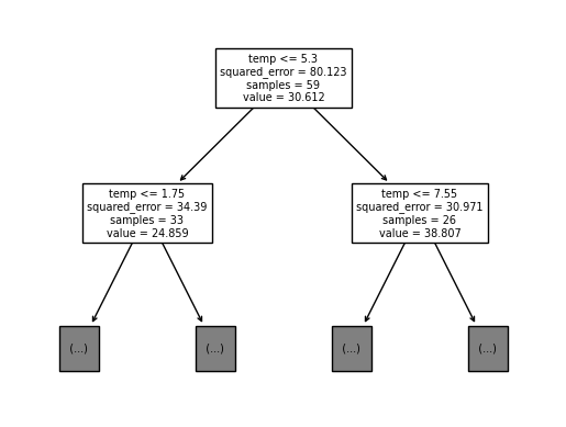
sklearn.tree.plot_tree(
    tree,
    feature_names=X.columns,
    max_depth=1
);
- tree 비교 (고정된 \(i\))
i=4
fig, ax = plt.subplots(2,1)
#---#
sklearn.tree.plot_tree(
    predictr.estimators_[i],
    feature_names=X.columns,
    max_depth=1,
    ax=ax[0]
)
ax[0].set_title('predictr.estimator')
#---#
my_tree = sklearn.tree.DecisionTreeRegressor()
my_tree.fit(X_array[samples[i]],y_array[samples[i]])
sklearn.tree.plot_tree(
    my_tree,
    feature_names=X.columns,
    max_depth=1,
    ax=ax[1]
);
ax[1].set_title('my_tree')
Text(0.5, 1.0, 'my_tree')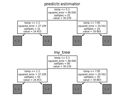
- tree 비교 (애니메이션)
fig, ax = plt.subplots(2,1)
plt.close()
#---#
def func(i):
    ax[0].clear()
    sklearn.tree.plot_tree(
        predictr.estimators_[i],
        feature_names=X.columns,
        max_depth=1,
        ax=ax[0]
    )
    ax[0].set_title('predictr.estimator')
    #---#
    ax[1].clear()
    my_tree = sklearn.tree.DecisionTreeRegressor()
    my_tree.fit(X_array[samples[i]],y_array[samples[i]])
    sklearn.tree.plot_tree(
        my_tree,
        feature_names=X.columns,
        max_depth=1,
        ax=ax[1]
    );
    ax[1].set_title('my_tree')
#---#
ani = matplotlib.animation.FuncAnimation(fig,func,frames=10)
display(IPython.display.HTML(ani.to_jshtml()))C. ReSampling + Fit
- 고정된 \(i\)
i=4
plt.plot(X,y,'o',alpha=0.2,color='gray')
plt.plot(X_array[samples[i]],y_array[samples[i]],'o',alpha=1/3)
plt.plot(X,trees[i].predict(X),'--')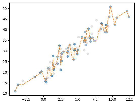
- 애니매이션
#---#
fig = plt.figure()
ax = fig.gca()
plt.close()
#---#
def func(i):
    ax.clear()
    ax.plot(X,y,'o',alpha=0.2,color='gray')
    ax.plot(X_array[samples[i]],y_array[samples[i]],'o',alpha=1/3)
    ax.plot(X,trees[i].predict(X),'--')
#---#
ani = matplotlib.animation.FuncAnimation(fig,func,frames=10)
display(IPython.display.HTML(ani.to_jshtml()))D. 앙상블결과 재현
- 최종결과물 (손으로..)
predictr.predict(X)array([11.88782962, 14.05941305, 15.02231867, 18.03161729, 19.62619066,
19.86214551, 15.84293717, 15.95940294, 15.95940294, 20.30137042,
20.30137042, 22.51278676, 22.51278676, 23.68899036, 20.7954938 ,
26.45727462, 26.45727462, 20.48421278, 20.48421278, 25.08188452,
25.08188452, 25.08188452, 31.42611771, 25.99393577, 25.99393577,
25.99393577, 27.05912187, 27.05912187, 29.60439358, 29.94005816,
29.18760881, 29.18760881, 30.75340115, 30.82608162, 32.48384789,
31.03678302, 29.02978839, 31.17487146, 31.17487146, 31.05349512,
29.147739 , 29.147739 , 29.147739 , 30.40843883, 30.40843883,
33.53154643, 34.26668831, 33.20982041, 33.20982041, 36.82818648,
36.82818648, 34.66545508, 34.66545508, 34.24047203, 33.0829342 ,
33.0829342 , 35.29894866, 35.50366771, 35.47938512, 35.47938512,
38.8116606 , 38.8116606 , 37.74794717, 34.84063828, 39.73515434,
40.01130524, 40.05274675, 41.9980937 , 42.26869452, 40.81707653,
40.16985211, 41.5373848 , 39.69311797, 42.97563198, 45.99122302,
49.35681519, 43.64765096, 45.32629064, 47.10042494, 46.28105912])np.stack([tree.predict(X) for tree in predictr.estimators_]).mean(axis=0)array([11.88782962, 14.05941305, 15.02231867, 18.03161729, 19.62619066,
19.86214551, 15.84293717, 15.95940294, 15.95940294, 20.30137042,
20.30137042, 22.51278676, 22.51278676, 23.68899036, 20.7954938 ,
26.45727462, 26.45727462, 20.48421278, 20.48421278, 25.08188452,
25.08188452, 25.08188452, 31.42611771, 25.99393577, 25.99393577,
25.99393577, 27.05912187, 27.05912187, 29.60439358, 29.94005816,
29.18760881, 29.18760881, 30.75340115, 30.82608162, 32.48384789,
31.03678302, 29.02978839, 31.17487146, 31.17487146, 31.05349512,
29.147739 , 29.147739 , 29.147739 , 30.40843883, 30.40843883,
33.53154643, 34.26668831, 33.20982041, 33.20982041, 36.82818648,
36.82818648, 34.66545508, 34.66545508, 34.24047203, 33.0829342 ,
33.0829342 , 35.29894866, 35.50366771, 35.47938512, 35.47938512,
38.8116606 , 38.8116606 , 37.74794717, 34.84063828, 39.73515434,
40.01130524, 40.05274675, 41.9980937 , 42.26869452, 40.81707653,
40.16985211, 41.5373848 , 39.69311797, 42.97563198, 45.99122302,
49.35681519, 43.64765096, 45.32629064, 47.10042494, 46.28105912])- 최종결과물 (코드로 정리)
def ensemble(trees,i=None):
    if i is None:
        i = len(trees)
    else:
        i = i+1
    yhat = np.stack([tree.predict(X) for tree in trees[:i]]).mean(axis=0)
return yhatensemble(trees,0) # 0번트리만 적용array([10.90026146, 10.90026146, 10.90026146, 19.46336233, 19.46336233,
20.31785349, 16.3076088 , 16.3076088 , 16.3076088 , 20.27763408,
20.27763408, 21.52796629, 21.52796629, 21.52796629, 18.34698175,
27.5369675 , 27.5369675 , 20.30881248, 20.30881248, 25.04963215,
25.04963215, 25.04963215, 32.42440294, 26.49340711, 26.49340711,
26.49340711, 26.40925726, 26.40925726, 29.55903213, 30.75418385,
29.70592592, 29.70592592, 31.45007539, 32.89828946, 32.89828946,
31.12503261, 25.9552363 , 33.12203011, 33.12203011, 30.60313283,
29.45886461, 29.45886461, 29.45886461, 30.60789344, 30.60789344,
30.60789344, 36.5245913 , 34.24458444, 34.24458444, 37.4829917 ,
37.4829917 , 37.4829917 , 37.4829917 , 31.13974993, 31.13974993,
31.13974993, 31.13974993, 36.58400962, 35.1723381 , 35.1723381 ,
39.75311187, 39.75311187, 39.75311187, 34.68877582, 44.47780794,
39.1744058 , 40.19626989, 42.86734269, 42.60143843, 40.80476673,
40.80476673, 42.1996627 , 38.72741866, 41.43992372, 45.95732063,
50.81374143, 42.30473921, 42.30473921, 48.7391566 , 46.00793717])ensemble(trees,1) # 0번트리,1번트리의 예측값 평균array([10.90026146, 12.45139248, 12.45139248, 18.56852168, 19.46336233,
20.31785349, 16.03419127, 16.57964463, 16.57964463, 21.02420483,
21.02420483, 21.3736233 , 21.3736233 , 23.07741787, 22.94197463,
27.5369675 , 27.5369675 , 19.83347885, 19.83347885, 26.16305209,
26.16305209, 26.16305209, 32.42440294, 28.7554569 , 28.7554569 ,
28.7554569 , 27.61337612, 27.61337612, 29.55903213, 30.75418385,
28.54972991, 28.54972991, 31.45007539, 30.82608162, 30.82608162,
31.66094517, 29.07604701, 32.65944392, 32.65944392, 30.60313283,
29.40787056, 29.40787056, 29.40787056, 30.5566788 , 30.5566788 ,
33.57934676, 36.5245913 , 35.63234869, 35.63234869, 37.25155232,
37.25155232, 35.85263528, 35.85263528, 32.46466946, 33.6755663 ,
33.6755663 , 35.78403852, 35.87817386, 35.1723381 , 35.1723381 ,
40.62427057, 40.62427057, 40.62427057, 34.68877582, 44.47780794,
41.82610687, 40.50051831, 41.83605471, 41.70310258, 40.80476673,
39.92694722, 40.6243952 , 40.08367119, 41.43992372, 43.69862217,
50.81374143, 42.30473921, 43.9833789 , 48.7391566 , 47.37354689])E. 학습과정 시각화
- 고정된 \(i\)
i=9
fig,ax = plt.subplots(1,4,figsize=(8,2))
#--#
ax[0].set_title("Step0")
ax[0].plot(X,y,'o',color='gray',alpha=0.2)
#--#
ax[1].set_title("Step1:ReSampling")
ax[1].plot(X,y,'o',color='gray',alpha=0.2)
ax[1].plot(X_array[samples[i]],y[samples[i]],'o',alpha=1/3)
#--#
ax[2].set_title("Step2:Fit")
ax[2].plot(X,y,'o',color='gray',alpha=0.2)
ax[2].plot(X_array[samples[i]],y[samples[i]],'o',alpha=1/3)
ax[2].plot(X,trees[i].predict(X),'--')
#--#
ax[3].set_title("Step3:Update(?)")
ax[3].plot(X,y,'o',color='gray',alpha=0.2)
ax[3].plot(X,ensemble(trees,i),'--',color='C1')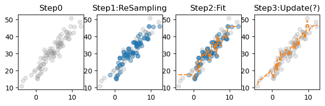
- 애니메이션
fig,ax = plt.subplots(1,4,figsize=(8,2))
plt.close()
#---#
def func(i):
    for a in ax:
        a.clear()
    #--#
    ax[0].set_title("Step0")
    ax[0].plot(X,y,'o',color='gray',alpha=0.2)
    #--#
    ax[1].set_title("Step1:ReSampling")
    ax[1].plot(X,y,'o',color='gray',alpha=0.2)
    ax[1].plot(X_array[samples[i]],y[samples[i]],'o',alpha=1/3)
    #--#
    ax[2].set_title("Step2:Fit")
    ax[2].plot(X,y,'o',color='gray',alpha=0.2)
    ax[2].plot(X_array[samples[i]],y[samples[i]],'o',alpha=1/3)
    ax[2].plot(X,trees[i].predict(X),'--')
    #--#
    ax[3].set_title("Step3:Update(?)")
    ax[3].plot(X,y,'o',color='gray',alpha=0.2)
    ax[3].plot(X,ensemble(trees,i),'--',color='C1')
#---#
ani = matplotlib.animation.FuncAnimation(fig,func,frames=10)
display(IPython.display.HTML(ani.to_jshtml()))6. Discussion
- 이런 방법을 생각한 근거? 부스트랩