07wk-30: 아이스크림(교호작용) / 회귀분석

1. 강의영상

2. Imports

import numpy as np
import pandas as pd 
import matplotlib.pyplot as plt 
import sklearn.linear_model 
import sklearn.tree
import sklearn.model_selection

3. 예비학습

df = pd.DataFrame({'X1':[2,3,4,1],'X2':['A','B','A','C']})
df 

	X1	X2
0	2	A
1	3	B
2	4	A
3	1	C

pd.get_dummies(df)

	X1	X2_A	X2_B	X2_C
0	2	True	False	False
1	3	False	True	False
2	4	True	False	False
3	1	False	False	True

• X2_A, X2_B, X2_C는 셋다 있을 필요는 없지 않나? –> 공선성문제가 생길수도 있음.

pd.get_dummies(df,drop_first=True)

	X1	X2_B	X2_C
0	2	False	False
1	3	True	False
2	4	False	False
3	1	False	True

4. Data

- load

np.random.seed(43052)
temp = pd.read_csv('https://raw.githubusercontent.com/guebin/DV2022/master/posts/temp.csv').iloc[:,3].to_numpy()[:100]
temp.sort()
choco = 40 + temp * 2.0 + np.random.randn(100)*3
vanilla = 60 + temp * 5.0 + np.random.randn(100)*3
df1 = pd.DataFrame({'temp':temp,'sales':choco}).assign(type='choco')
df2 = pd.DataFrame({'temp':temp,'sales':vanilla}).assign(type='vanilla')
df_train = pd.concat([df1,df2])
df_train

	temp	sales	type
0	-4.1	32.950261	choco
1	-3.7	35.852524	choco
2	-3.0	37.428335	choco
3	-1.3	38.323681	choco
4	-0.5	39.713362	choco
...	...	...	...
95	12.4	119.708075	vanilla
96	13.4	129.300464	vanilla
97	14.7	136.596568	vanilla
98	15.0	136.213140	vanilla
99	15.2	135.595252	vanilla

200 rows × 3 columns

- 시각화 및 해석

plt.plot(df_train[df.type=='choco'].temp,df_train[df.type=='choco'].sales,'o',label='choco')
plt.plot(df_train[df.type=='vanilla'].temp,df_train[df.type=='vanilla'].sales,'o',label='vanilla')
plt.legend()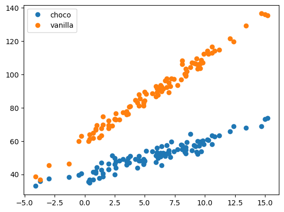

• 온도에 따른 아이스크림 판매량이 아이스크림의 tpye에 따라 동일하다면 기울기가 동일하고 절편이 다른 두 직선이 나올것임.
• 하지만 현재는 초코보다 바닐라맛이 기온의 영향을 많이 받아보임 \(\to\) (바닐라아이스크림,온도)는 (초코아이스크림,온도)보다 궁합이 좋다. \(\to\) 아이스크림 type과 온도사이에는 교호작용이 존재한다.

5. 분석1

- 분석1: 모형을 아래와 같이 본다.

• \({\bf X}\): temp, type
• \({\bf y}\): sales

# step1 
X,y = pd.get_dummies(df_train[['temp','type']],drop_first=True), df['sales']
# step2
predictr = sklearn.linear_model.LinearRegression()
# step3
predictr.fit(X,y)
# step4 
df_train['sales_hat'] = predictr.predict(X)

predictr.score(X,y)

0.9249530603100549

• 점수가 잘나왔다고 너무 좋아하지 마세요.
• 시각화를 반드시 해보고 더 맞출수 있는 여지가 있는지 항상 확인할 것

plt.plot(df_train[df.type=='choco'].temp,df_train[df.type=='choco'].sales,'o',label='choco',color='C0',alpha=0.5)
plt.plot(df_train[df.type=='choco'].temp,df_train[df.type=='choco'].sales_hat,'--',color='C0')
plt.plot(df_train[df.type=='vanilla'].temp,df_train[df.type=='vanilla'].sales,'o',label='vanilla',color='C1',alpha=0.5)
plt.plot(df_train[df.type=='vanilla'].temp,df_train[df.type=='vanilla'].sales_hat,'--',color='C1')
plt.legend()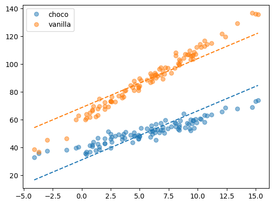

이 모형은 초코/바닐라에 대한 기울기차이를 “표현”할 수 없다. 이러한 상황은 “모형의 표현력이 약하다” 혹은 “언더피팅”인 상황이라고 한다.

6. 분석2

- 모형을 아래와 같이 본다.

• \({\bf X}\): temp, type, temp \(\times\) type
• \({\bf y}\): sales

pd.get_dummies(df_train[['temp','type']],drop_first=True).eval('interaction = temp*type_vanilla')

	temp	type_vanilla	interaction
0	-4.1	False	-0.0
1	-3.7	False	-0.0
2	-3.0	False	-0.0
3	-1.3	False	-0.0
4	-0.5	False	-0.0
...	...	...	...
95	12.4	True	12.4
96	13.4	True	13.4
97	14.7	True	14.7
98	15.0	True	15.0
99	15.2	True	15.2

200 rows × 3 columns

# step1 
X = pd.get_dummies(df_train[['temp','type']],drop_first=True).eval('interaction = temp*type_vanilla')
y = df['sales']
# step2
predictr = sklearn.linear_model.LinearRegression()
# step3
predictr.fit(X,y)
# step4 
df_train['sales_hat'] = predictr.predict(X)

predictr.score(X,y)

0.9865793819066231

plt.plot(df_train[df.type=='choco'].temp,df_train[df.type=='choco'].sales,'o',label='choco',color='C0',alpha=0.5)
plt.plot(df_train[df.type=='choco'].temp,df_train[df.type=='choco'].sales_hat,'--',color='C0')
plt.plot(df_train[df.type=='vanilla'].temp,df_train[df.type=='vanilla'].sales,'o',label='vanilla',color='C1',alpha=0.5)
plt.plot(df_train[df.type=='vanilla'].temp,df_train[df.type=='vanilla'].sales_hat,'--',color='C1')
plt.legend()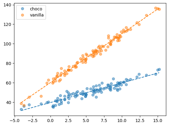

Note: 초코/바닐라에 대한 절편차이는 type로, 초코/바닐라에 대한 기울기 차이는 temp\(\times\)type로 표현한다.