import numpy as np
import pandas as pd
import matplotlib.pyplot as plt
import sklearn.linear_model
#---#
import warnings
warnings.filterwarnings('ignore')06wk-25: 취업(다중공선성) / Lasso
1. 강의영상
2. Imports
3. Data
df = pd.read_csv("https://raw.githubusercontent.com/guebin/MP2023/main/posts/employment_multicollinearity.csv")
np.random.seed(43052)
df['employment_score'] = df.gpa * 1.0 + df.toeic* 1/100 + np.random.randn(500)df| employment_score | gpa | toeic | toeic0 | toeic1 | toeic2 | toeic3 | toeic4 | toeic5 | toeic6 | ... | toeic490 | toeic491 | toeic492 | toeic493 | toeic494 | toeic495 | toeic496 | toeic497 | toeic498 | toeic499 | |
|---|---|---|---|---|---|---|---|---|---|---|---|---|---|---|---|---|---|---|---|---|---|
| 0 | 1.784955 | 0.051535 | 135 | 129.566309 | 133.078481 | 121.678398 | 113.457366 | 133.564200 | 136.026566 | 141.793547 | ... | 132.014696 | 140.013265 | 135.575816 | 143.863346 | 152.162740 | 132.850033 | 115.956496 | 131.842126 | 125.090801 | 143.568527 |
| 1 | 10.789671 | 0.355496 | 935 | 940.563187 | 935.723570 | 939.190519 | 938.995672 | 945.376482 | 927.469901 | 952.424087 | ... | 942.251184 | 923.241548 | 939.924802 | 921.912261 | 953.250300 | 931.743615 | 940.205853 | 930.575825 | 941.530348 | 934.221055 |
| 2 | 8.221213 | 2.228435 | 485 | 493.671390 | 493.909118 | 475.500970 | 480.363752 | 478.868942 | 493.321602 | 490.059102 | ... | 484.438233 | 488.101275 | 485.626742 | 475.330715 | 485.147363 | 468.553780 | 486.870976 | 481.640957 | 499.340808 | 488.197332 |
| 3 | 2.137594 | 1.179701 | 65 | 62.272565 | 55.957257 | 68.521468 | 76.866765 | 51.436321 | 57.166824 | 67.834920 | ... | 67.653225 | 65.710588 | 64.146780 | 76.662194 | 66.837839 | 82.379018 | 69.174745 | 64.475993 | 52.647087 | 59.493275 |
| 4 | 8.650144 | 3.962356 | 445 | 449.280637 | 438.895582 | 433.598274 | 444.081141 | 437.005100 | 434.761142 | 443.135269 | ... | 455.940348 | 435.952854 | 441.521145 | 443.038886 | 433.118847 | 466.103355 | 430.056944 | 423.632873 | 446.973484 | 442.793633 |
| ... | ... | ... | ... | ... | ... | ... | ... | ... | ... | ... | ... | ... | ... | ... | ... | ... | ... | ... | ... | ... | ... |
| 495 | 9.057243 | 4.288465 | 280 | 276.680902 | 274.502675 | 277.868536 | 292.283300 | 277.476630 | 281.671647 | 296.307373 | ... | 269.541846 | 278.220546 | 278.484758 | 284.901284 | 272.451612 | 265.784490 | 275.795948 | 280.465992 | 268.528889 | 283.638470 |
| 496 | 4.108020 | 2.601212 | 310 | 296.940263 | 301.545000 | 306.725610 | 314.811407 | 311.935810 | 309.695838 | 301.979914 | ... | 304.680578 | 295.476836 | 316.582100 | 319.412132 | 312.984039 | 312.372112 | 312.106944 | 314.101927 | 309.409533 | 297.429968 |
| 497 | 2.430590 | 0.042323 | 225 | 206.793217 | 228.335345 | 222.115146 | 216.479498 | 227.469560 | 238.710310 | 233.797065 | ... | 233.469238 | 235.160919 | 228.517306 | 228.349646 | 224.153606 | 230.860484 | 218.683195 | 232.949484 | 236.951938 | 227.997629 |
| 498 | 5.343171 | 1.041416 | 320 | 327.461442 | 323.019899 | 329.589337 | 313.312233 | 315.645050 | 324.448247 | 314.271045 | ... | 326.297700 | 309.893822 | 312.873223 | 322.356584 | 319.332809 | 319.405283 | 324.021917 | 312.363694 | 318.493866 | 310.973930 |
| 499 | 6.505106 | 3.626883 | 375 | 370.966595 | 364.668477 | 371.853566 | 373.574930 | 376.701708 | 356.905085 | 354.584022 | ... | 382.278782 | 379.460816 | 371.031640 | 370.272639 | 375.618182 | 369.252740 | 376.925543 | 391.863103 | 368.735260 | 368.520844 |
500 rows × 503 columns
4. True (Oracle)
## step1
df_train, df_test = sklearn.model_selection.train_test_split(df,test_size=0.3,random_state=42)
X = df_train.loc[:,'gpa':'toeic']
y = df_train[['employment_score']]
XX = df_test.loc[:,'gpa':'toeic']
yy = df_test[['employment_score']]
## step2
predictr = sklearn.linear_model.LinearRegression()
## step3
predictr.fit(X,y)
## step4 : pass LinearRegression()In a Jupyter environment, please rerun this cell to show the HTML representation or trust the notebook.
On GitHub, the HTML representation is unable to render, please try loading this page with nbviewer.org.
LinearRegression()
print(f'train_score:\t{predictr.score(X,y):.4f}')
print(f'test_score:\t{predictr.score(XX,yy):.4f}')
train_score: 0.9133
test_score: 0.91275. Baseline
- 모든 변수를 활용하여 회귀모형으로 적합 \(\to\) 최악의 결과
## step1
df_train, df_test = sklearn.model_selection.train_test_split(df,test_size=0.3,random_state=42)
X = df_train.loc[:,'gpa':'toeic499']
y = df_train[['employment_score']]
XX = df_test.loc[:,'gpa':'toeic499']
yy = df_test[['employment_score']]
## step2
predictr = sklearn.linear_model.LinearRegression()
## step3
predictr.fit(X,y)
## step4 : pass LinearRegression()In a Jupyter environment, please rerun this cell to show the HTML representation or trust the notebook.
On GitHub, the HTML representation is unable to render, please try loading this page with nbviewer.org.
LinearRegression()
- 평가
print(f'train_score:\t {predictr.score(X,y):.4f}')
print(f'test_score:\t {predictr.score(XX,yy):.4f}')
train_score: 1.0000
test_score: 0.11716. Lasso
- Lasso를 이용
## step1
df_train, df_test = sklearn.model_selection.train_test_split(df,test_size=0.3,random_state=42)
X = df_train.loc[:,'gpa':'toeic499']
y = df_train[['employment_score']]
XX = df_test.loc[:,'gpa':'toeic499']
yy = df_test[['employment_score']]
## step2
predictr = sklearn.linear_model.Lasso(alpha=1)
## step3
predictr.fit(X,y)
## step4 : pass Lasso(alpha=1)In a Jupyter environment, please rerun this cell to show the HTML representation or trust the notebook.
On GitHub, the HTML representation is unable to render, please try loading this page with nbviewer.org.
Lasso(alpha=1)
- 평가
print(f'train_score:\t {predictr.score(X,y):.4f}')
print(f'test_score:\t {predictr.score(XX,yy):.4f}')
train_score: 0.8600
test_score: 0.83067. Lasso는 왜 결과를 좋게 만들까?
A. 정확한 설명
- 어려워요..
B. 직관적 설명 (엄밀하지 않은 설명)
- 느낌: 몇 개의 toeic coef들로 쉽게 0.01을 만들게 해서는 안된다.
- 아이디어1: 0.01을 동일한 값으로 균등하게 배분한다. – Ridge, L2-penalty
- 아이디어2: 아주 적은숫자의 coef만을 살려두고 나머지 coef값은 0으로 강제한다. – Lasso, L1-penalty
- 계수값이 0이라는 의미: 그 변수를 제거한것과 같은 효과
- 아이디어2의 기원: y ~ toeic + gpa 가 트루이지만, y ~ toeic0 + gpa 으로 적합해도 괜찮잖아?
- 진짜 학습된 계수값이 대부분 0인지 확인해보자.
plt.plot(predictr.coef_[1:])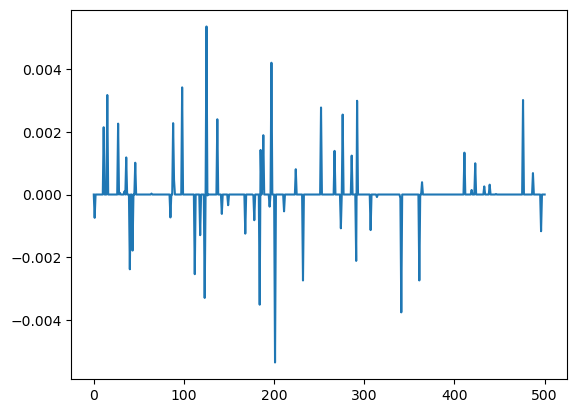
C. \(\alpha\) 에 따른 변화 관찰
- 여러개의 predictor 학습
## step1
df_train, df_test = sklearn.model_selection.train_test_split(df,test_size=0.3,random_state=42)
X = df_train.loc[:,'gpa':'toeic499']
y = df_train[['employment_score']]
XX = df_test.loc[:,'gpa':'toeic499']
yy = df_test[['employment_score']]
## step2
alphas = np.linspace(0,2,100)
predictrs = [sklearn.linear_model.Lasso(alpha=alpha) for alpha in alphas]
## step3
for predictr in predictrs:
    predictr.fit(X,y)
## step4 : pass plt.plot(predictrs[0].coef_[1:],label=r'$\alpha={}$'.format(predictrs[0].alpha))
plt.plot(predictrs[50].coef_[1:],label=r'$\alpha={}$'.format(predictrs[50].alpha))
plt.plot(predictrs[-1].coef_[1:],label=r'$\alpha={}$'.format(predictrs[-1].alpha))
plt.legend()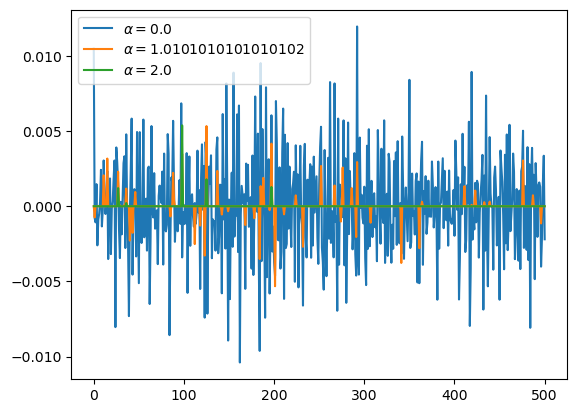
- predictor 들의 toeic 계수합은 여전히 0.01 근처
print(f'alpha={predictrs[0].alpha:.4f}\tsum(toeic_coef)={predictrs[0].coef_[1:].sum()}')
print(f'alpha={predictrs[50].alpha:.4f}\tsum(toeic_coef)={predictrs[50].coef_[1:].sum()}')
print(f'alpha={predictrs[-1].alpha:.4f}\tsum(toeic_coef)={predictrs[-1].coef_[1:].sum()}')
alpha=0.0000 sum(toeic_coef)=0.010291301406468518
alpha=1.0101 sum(toeic_coef)=0.009986115762478664
alpha=2.0000 sum(toeic_coef)=0.009864586871194559- number of non-zero coefs 를 시각화
non_zero_coefs = [(abs(predictr.coef_[1:])>0).sum() for predictr in predictrs]plt.plot(alphas,non_zero_coefs)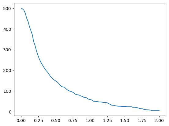
D. coef를 0으로 만드는 수학적 장치
- Ridge(복습): coef의 값들을 엔빵하는 수학적 장치
- 패널티: 유사토익들의 계수값을 제곱한뒤 합치고(=L2-norm을 구하고), 그 값이 0에서 떨어져 있을 수록 패널티를 줄꺼야!
- Lasso: coef의 값들을 대부분 0으로 만드는 수학적 장치
- 패널티: 유사토익들의 계수값의 절대값을 구한뒤에 합치고(=L1-norm을 구하고), 그 값이 0에서 떨어져 있을 수록 패널티를 줄꺼야!
- 사실 L1, L2 패널티에 따라서 이러한 결과가 나오는 것은 이해하기 어렵다. (그래서 취업/대학원 진학시 단골질문중 하나)