import numpy as np
import pandas as pd
import matplotlib.pyplot as plt
import sklearn.linear_model06wk-23: 취업(다중공선성) / Ridge – 추가해설
1. 강의영상
2. Imports
3. Data
df = pd.read_csv("https://raw.githubusercontent.com/guebin/MP2023/main/posts/employment_multicollinearity.csv")
np.random.seed(43052)
df['employment_score'] = df.gpa * 1.0 + df.toeic* 1/100 + np.random.randn(500)df| employment_score | gpa | toeic | toeic0 | toeic1 | toeic2 | toeic3 | toeic4 | toeic5 | toeic6 | ... | toeic490 | toeic491 | toeic492 | toeic493 | toeic494 | toeic495 | toeic496 | toeic497 | toeic498 | toeic499 | |
|---|---|---|---|---|---|---|---|---|---|---|---|---|---|---|---|---|---|---|---|---|---|
| 0 | 1.784955 | 0.051535 | 135 | 129.566309 | 133.078481 | 121.678398 | 113.457366 | 133.564200 | 136.026566 | 141.793547 | ... | 132.014696 | 140.013265 | 135.575816 | 143.863346 | 152.162740 | 132.850033 | 115.956496 | 131.842126 | 125.090801 | 143.568527 |
| 1 | 10.789671 | 0.355496 | 935 | 940.563187 | 935.723570 | 939.190519 | 938.995672 | 945.376482 | 927.469901 | 952.424087 | ... | 942.251184 | 923.241548 | 939.924802 | 921.912261 | 953.250300 | 931.743615 | 940.205853 | 930.575825 | 941.530348 | 934.221055 |
| 2 | 8.221213 | 2.228435 | 485 | 493.671390 | 493.909118 | 475.500970 | 480.363752 | 478.868942 | 493.321602 | 490.059102 | ... | 484.438233 | 488.101275 | 485.626742 | 475.330715 | 485.147363 | 468.553780 | 486.870976 | 481.640957 | 499.340808 | 488.197332 |
| 3 | 2.137594 | 1.179701 | 65 | 62.272565 | 55.957257 | 68.521468 | 76.866765 | 51.436321 | 57.166824 | 67.834920 | ... | 67.653225 | 65.710588 | 64.146780 | 76.662194 | 66.837839 | 82.379018 | 69.174745 | 64.475993 | 52.647087 | 59.493275 |
| 4 | 8.650144 | 3.962356 | 445 | 449.280637 | 438.895582 | 433.598274 | 444.081141 | 437.005100 | 434.761142 | 443.135269 | ... | 455.940348 | 435.952854 | 441.521145 | 443.038886 | 433.118847 | 466.103355 | 430.056944 | 423.632873 | 446.973484 | 442.793633 |
| ... | ... | ... | ... | ... | ... | ... | ... | ... | ... | ... | ... | ... | ... | ... | ... | ... | ... | ... | ... | ... | ... |
| 495 | 9.057243 | 4.288465 | 280 | 276.680902 | 274.502675 | 277.868536 | 292.283300 | 277.476630 | 281.671647 | 296.307373 | ... | 269.541846 | 278.220546 | 278.484758 | 284.901284 | 272.451612 | 265.784490 | 275.795948 | 280.465992 | 268.528889 | 283.638470 |
| 496 | 4.108020 | 2.601212 | 310 | 296.940263 | 301.545000 | 306.725610 | 314.811407 | 311.935810 | 309.695838 | 301.979914 | ... | 304.680578 | 295.476836 | 316.582100 | 319.412132 | 312.984039 | 312.372112 | 312.106944 | 314.101927 | 309.409533 | 297.429968 |
| 497 | 2.430590 | 0.042323 | 225 | 206.793217 | 228.335345 | 222.115146 | 216.479498 | 227.469560 | 238.710310 | 233.797065 | ... | 233.469238 | 235.160919 | 228.517306 | 228.349646 | 224.153606 | 230.860484 | 218.683195 | 232.949484 | 236.951938 | 227.997629 |
| 498 | 5.343171 | 1.041416 | 320 | 327.461442 | 323.019899 | 329.589337 | 313.312233 | 315.645050 | 324.448247 | 314.271045 | ... | 326.297700 | 309.893822 | 312.873223 | 322.356584 | 319.332809 | 319.405283 | 324.021917 | 312.363694 | 318.493866 | 310.973930 |
| 499 | 6.505106 | 3.626883 | 375 | 370.966595 | 364.668477 | 371.853566 | 373.574930 | 376.701708 | 356.905085 | 354.584022 | ... | 382.278782 | 379.460816 | 371.031640 | 370.272639 | 375.618182 | 369.252740 | 376.925543 | 391.863103 | 368.735260 | 368.520844 |
500 rows × 503 columns
4. True
- 신이라면 (=데이터가 만들어진 비밀을 알고 있다면) 아래와 같이 했을 것
## step1 --- toeic, gpa 만 남기고 나머지 변수를 삭제
df_train, df_test = sklearn.model_selection.train_test_split(df,test_size=0.3,random_state=42)
X = df_train.loc[:,'gpa':'toeic']
y = df_train.loc[:,'employment_score']
XX = df_test.loc[:,'gpa':'toeic']
yy = df_test.loc[:,'employment_score']
## step2
predictr = sklearn.linear_model.LinearRegression()
## step3
predictr.fit(X,y)
## step4 -- pass LinearRegression()In a Jupyter environment, please rerun this cell to show the HTML representation or trust the notebook.
On GitHub, the HTML representation is unable to render, please try loading this page with nbviewer.org.
LinearRegression()
- 평가
print(f'train_score: {predictr.score(X,y):.4f}')
print(f'test_score: {predictr.score(XX,yy):.4f}')
train_score: 0.9133
test_score: 0.91275. Baseline
- 모든 변수를 활용하여 회귀모형으로 적합 \(\to\) 최악의 결과
## step1 --- toeic, gpa 만 남기고 나머지 변수를 삭제
df_train, df_test = sklearn.model_selection.train_test_split(df,test_size=0.3,random_state=42)
X = df_train.loc[:,'gpa':'toeic499']
y = df_train.loc[:,'employment_score']
XX = df_test.loc[:,'gpa':'toeic499']
yy = df_test.loc[:,'employment_score']
## step2
predictr = sklearn.linear_model.LinearRegression()
## step3
predictr.fit(X,y)
## step4 -- pass LinearRegression()In a Jupyter environment, please rerun this cell to show the HTML representation or trust the notebook.
On GitHub, the HTML representation is unable to render, please try loading this page with nbviewer.org.
LinearRegression()
- 평가
print(f'train_score: {predictr.score(X,y):.4f}')
print(f'test_score: {predictr.score(XX,yy):.4f}')
train_score: 1.0000
test_score: 0.11716. Ridge
- 통계학자에게 자문: 이럴 경우 Ridge를 사용하면 됩니다..
## step1 --- toeic, gpa 만 남기고 나머지 변수를 삭제
df_train, df_test = sklearn.model_selection.train_test_split(df,test_size=0.3,random_state=42)
X = df_train.loc[:,'gpa':'toeic499']
y = df_train.loc[:,'employment_score']
XX = df_test.loc[:,'gpa':'toeic499']
yy = df_test.loc[:,'employment_score']
## step2
predictr = sklearn.linear_model.Ridge(alpha=1) # sklearn.linear_model.Ridge()와 같은코드
## step3
predictr.fit(X,y)
## step4 -- pass Ridge(alpha=1)In a Jupyter environment, please rerun this cell to show the HTML representation or trust the notebook.
On GitHub, the HTML representation is unable to render, please try loading this page with nbviewer.org.
Ridge(alpha=1)
- 평가: 안되는데요..??
print(f'train_score: {predictr.score(X,y):.4f}')
print(f'test_score: {predictr.score(XX,yy):.4f}')
train_score: 1.0000
test_score: 0.1173- 하이퍼 파라메터 튜닝 \(\alpha=1.5\)
## step1 --- toeic, gpa 만 남기고 나머지 변수를 삭제
df_train, df_test = sklearn.model_selection.train_test_split(df,test_size=0.3,random_state=42)
X = df_train.loc[:,'gpa':'toeic499']
y = df_train.loc[:,'employment_score']
XX = df_test.loc[:,'gpa':'toeic499']
yy = df_test.loc[:,'employment_score']
## step2
predictr = sklearn.linear_model.Ridge(alpha=1.5)
## step3
predictr.fit(X,y)
## step4 -- pass
#---#
print(f'train_score: {predictr.score(X,y):.4f}')
print(f'test_score: {predictr.score(XX,yy):.4f}')
train_score: 1.0000
test_score: 0.1174- 조금 나아진것 같기도?
- 하이퍼 파라메터 튜닝 \(\alpha=5e8\)
## step1 --- toeic, gpa 만 남기고 나머지 변수를 삭제
df_train, df_test = sklearn.model_selection.train_test_split(df,test_size=0.3,random_state=42)
X = df_train.loc[:,'gpa':'toeic499']
y = df_train.loc[:,'employment_score']
XX = df_test.loc[:,'gpa':'toeic499']
yy = df_test.loc[:,'employment_score']
## step2
predictr = sklearn.linear_model.Ridge(alpha=5e8)
## step3
predictr.fit(X,y)
## step4 -- pass
#---#
print(f'train_score: {predictr.score(X,y):.4f}')
print(f'test_score: {predictr.score(XX,yy):.4f}')
train_score: 0.7507
test_score: 0.7438- 오라클에 비할바는 아니긴한데 공선성이 있는 경우라도 Ridge에서 적절한 alpha를 고른다면 망하는 모형을 만들진 않음
7. Ridge는 왜 결과를 좋게 만들까?
A. 정확한 설명
- SVD를 이용하여 이론적인 계산하면 sklearn.linear_model.LinearRegression()로 적합한 결과보다 sklearn.linear_model.Ridge()로 적합한 결과를 더 좋게 만드는 \(\alpha\)가 항상 존재함을 증명할 수 있음.
B. 직관적 설명 (엄밀하지 않은 설명)
Step1: LinearRegression은 왜 망했는가?
- 토익의 계수는 실제로 \(\frac{1}{100}\)이다. 적딩히
toeic_coef+ … +toeic499_coef\(\approx\) 0.01 이라면
대충 맞는 답이다.
## step1 --- toeic, gpa 만 남기고 나머지 변수를 삭제
df_train, df_test = sklearn.model_selection.train_test_split(df,test_size=0.3,random_state=42)
X = df_train.loc[:,'gpa':'toeic499']
y = df_train.loc[:,'employment_score']
XX = df_test.loc[:,'gpa':'toeic499']
yy = df_test.loc[:,'employment_score']
## step2
predictr = sklearn.linear_model.LinearRegression()
## step3
predictr.fit(X,y)
## step4 -- pass
#---#
print(f'train_score: {predictr.score(X,y):.4f}')
print(f'test_score: {predictr.score(XX,yy):.4f}')
train_score: 1.0000
test_score: 0.1171s= pd.Series(predictr.coef_)
s.index = X.columns
s[1:].sum()0.010302732920632579- 그런데 사실 저 0.01이라는 값은 몇개의 계수만 있어도 만들 수 있다. (toeic2와 toeic3에 해당하는 계수)
s['toeic2']+s['toeic3']0.010142832986793252- 이런논리로 치면 toeic2, toeic3에 해당하는 계수만 있다면 사실 \(y\)를 설명하는데 충분했고, 나머지는 불필요한 특징이 된다. (그리고 불필요한 특징은 오버피팅을 유발한다)
Step2: Ridge의 아이디어
- Ridge의 아이디어: toeic2, toeic3 와 같이 몇개의 변수로만 0.01이라는 수를 설명할 수 없도록 “강제”하자. 즉 몇개의 변수로만 0.01이라는 수를 설명할 수 없도록 “패널티”를 주자.
- 패널티: 유사토익들의 계수값을 제곱한뒤 합치고(=L2-norm을 구하고), 그 값이 0에서 떨어져 있을 수록 패널티를 줄꺼야!
- 이러한 패널티를 줄 경우 결과적으로 0.01의 값이 “동일하게 나누어져서” 나오는 값(=\(\frac{1}{100}\frac{1}{501}\))이 계수값으로 추정된다. (왜? – 요건 정확하게 이해하는게 사실 지금은 힘듬)
- 잘 적용된 Ridge의 결과를 보면 아래와 같이 계수값이 저장되어 있음.
## step1 --- toeic, gpa 만 남기고 나머지 변수를 삭제
df_train, df_test = sklearn.model_selection.train_test_split(df,test_size=0.3,random_state=42)
X = df_train.loc[:,'gpa':'toeic499']
y = df_train.loc[:,'employment_score']
XX = df_test.loc[:,'gpa':'toeic499']
yy = df_test.loc[:,'employment_score']
## step2
predictr = sklearn.linear_model.Ridge(alpha=5e8)
## step3
predictr.fit(X,y)
## step4 -- pass
#---#
print(f'train_score: {predictr.score(X,y):.4f}')
print(f'test_score: {predictr.score(XX,yy):.4f}')
train_score: 0.7507
test_score: 0.7438s = pd.Series(predictr.coef_)
s.index = X.columns
sgpa 0.000001
toeic 0.000019
toeic0 0.000018
toeic1 0.000018
toeic2 0.000019
...
toeic495 0.000018
toeic496 0.000019
toeic497 0.000019
toeic498 0.000019
toeic499 0.000019
Length: 502, dtype: float640.01/5011.9960079840319362e-05- 결국 Ridge를 사용하면 계수들의 값이 “동일하게 나누어지는” 효과가 나타남
2023-10-24 추가해설
모든 계수가 “엔빵”된다는 의미는 아니에요. 예를들어 X1=toeic, X2≈toeic*2 라면?
- 패널티를 주는 정도? \(\alpha\)로 조절함.. \(\alpha\)를 크게 할수록 패널티를 많이줌
C. \(\alpha\)에 따른 계수값 변화
- 여러개의 predictor 학습
## step1 --- toeic, gpa 만 남기고 나머지 변수를 삭제
df_train, df_test = sklearn.model_selection.train_test_split(df,test_size=0.3,random_state=42)
X = df_train.loc[:,'gpa':'toeic499']
y = df_train.loc[:,'employment_score']
XX = df_test.loc[:,'gpa':'toeic499']
yy = df_test.loc[:,'employment_score']
## step2
alphas = [5e2, 5e3, 5e4, 5e5, 5e6, 5e7, 5e8]
predictrs = [sklearn.linear_model.Ridge(alpha=alpha) for alpha in alphas]
## step3
for predictr in predictrs:
    predictr.fit(X,y)
## step4 -- pass
- 계수값 시각화
predictrs[0].alpha500.0plt.plot(predictrs[0].coef_[1:],label=r'$\alpha$={}'.format(predictrs[0].alpha))
plt.plot(predictrs[3].coef_[1:],label=r'$\alpha$={}'.format(predictrs[1].alpha))
plt.legend()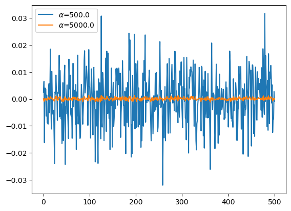
plt.plot(predictrs[3].coef_[1:],label=r'$\alpha$={}'.format(predictrs[3].alpha))
plt.plot(predictrs[5].coef_[1:],label=r'$\alpha$={}'.format(predictrs[5].alpha))
plt.legend()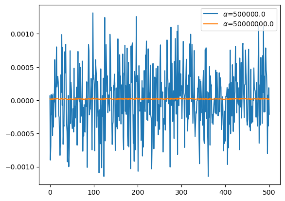
plt.plot(predictrs[5].coef_[1:],label=r'$\alpha$={}'.format(predictrs[5].alpha))
plt.plot(predictrs[-1].coef_[1:],label=r'$\alpha$={}'.format(predictrs[-1].alpha))
plt.legend()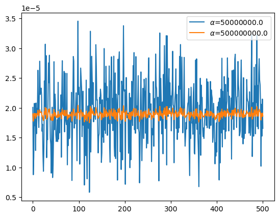
- 직관: 마지막 predictor의 계수값을 살펴보자.
predictrs[-1].coef_array([1.10421248e-06, 1.89938091e-05, 1.77768343e-05, 1.82118332e-05,
1.90895673e-05, 1.87128138e-05, 1.90343037e-05, 1.82483251e-05,
1.90405022e-05, 1.85802628e-05, 1.90021086e-05, 1.88952130e-05,
1.96003229e-05, 1.89154663e-05, 1.86638217e-05, 1.92666606e-05,
1.97107043e-05, 1.92214868e-05, 1.92961317e-05, 1.93321368e-05,
1.92194541e-05, 1.85663279e-05, 1.86805137e-05, 1.81649873e-05,
1.78656367e-05, 1.83171419e-05, 1.94428947e-05, 1.89710925e-05,
2.00598946e-05, 1.88384883e-05, 1.98903125e-05, 1.81113551e-05,
1.85043847e-05, 1.84424971e-05, 1.91508275e-05, 1.97427867e-05,
1.93598061e-05, 1.98264264e-05, 1.89934042e-05, 1.84770850e-05,
1.83617634e-05, 1.79346774e-05, 1.84943159e-05, 1.89803006e-05,
1.78633749e-05, 1.80073666e-05, 1.85664525e-05, 1.97390143e-05,
1.86574281e-05, 1.92233226e-05, 1.91281904e-05, 1.85617627e-05,
1.83939489e-05, 1.84309427e-05, 1.88142167e-05, 1.84159665e-05,
1.94078579e-05, 1.84515402e-05, 1.88107980e-05, 1.85889903e-05,
1.89357356e-05, 1.88750847e-05, 1.92107444e-05, 1.81799279e-05,
1.92122152e-05, 1.97863670e-05, 1.89851436e-05, 1.88974919e-05,
1.88566578e-05, 1.95841935e-05, 1.86398380e-05, 1.95801159e-05,
1.87550098e-05, 1.87392625e-05, 1.87462595e-05, 1.96056001e-05,
1.80626630e-05, 1.88237701e-05, 1.83108446e-05, 1.88087164e-05,
1.84723703e-05, 1.84767748e-05, 1.89267252e-05, 1.87604297e-05,
1.86945591e-05, 1.92924236e-05, 1.77843453e-05, 1.85415541e-05,
1.91448999e-05, 1.98281375e-05, 1.97994651e-05, 1.86653004e-05,
1.87298830e-05, 1.87474975e-05, 1.90018315e-05, 1.92043808e-05,
1.88941675e-05, 1.81646176e-05, 1.91508494e-05, 2.04322537e-05,
1.92111546e-05, 1.93061022e-05, 1.92088349e-05, 1.80206353e-05,
1.89399818e-05, 1.96895533e-05, 1.94410839e-05, 1.92051217e-05,
1.84961416e-05, 1.89785667e-05, 1.92235780e-05, 1.86729143e-05,
1.88439733e-05, 1.76776615e-05, 1.87493841e-05, 1.86986837e-05,
1.81917859e-05, 1.94657238e-05, 1.82063420e-05, 1.78143049e-05,
1.88432683e-05, 1.90674860e-05, 1.86411824e-05, 1.93286721e-05,
1.75163829e-05, 1.86852659e-05, 2.02343956e-05, 1.82025623e-05,
1.89153395e-05, 1.98862774e-05, 1.94775038e-05, 1.90665531e-05,
1.94170642e-05, 1.88227118e-05, 1.88792179e-05, 1.89712787e-05,
1.87855482e-05, 1.87895464e-05, 2.00798925e-05, 1.97167119e-05,
1.91644137e-05, 1.90990710e-05, 1.85836048e-05, 1.82346595e-05,
1.85731253e-05, 1.84871242e-05, 1.90728256e-05, 1.90277156e-05,
1.93085319e-05, 1.91719254e-05, 1.80097271e-05, 1.82517485e-05,
1.90904218e-05, 1.85232604e-05, 1.88184612e-05, 1.84002976e-05,
2.00337440e-05, 1.86478638e-05, 1.93507546e-05, 1.85547358e-05,
1.97154574e-05, 1.91189346e-05, 1.93320777e-05, 1.85313268e-05,
1.91085306e-05, 1.88406812e-05, 1.87444892e-05, 1.96637559e-05,
1.83552699e-05, 1.80759243e-05, 1.94662845e-05, 1.93761303e-05,
1.98339288e-05, 1.87139235e-05, 1.91131387e-05, 1.85801855e-05,
1.91544816e-05, 1.98413649e-05, 1.84027849e-05, 1.81842651e-05,
1.95888229e-05, 1.80738476e-05, 1.92457286e-05, 1.91474170e-05,
1.88737956e-05, 1.78029998e-05, 1.97734483e-05, 1.92409710e-05,
1.97346045e-05, 1.99425451e-05, 1.89157923e-05, 1.82538525e-05,
1.87475300e-05, 1.79663692e-05, 1.94360535e-05, 1.93333725e-05,
1.81368431e-05, 1.91860664e-05, 2.03648683e-05, 1.92870391e-05,
1.92561212e-05, 1.92408929e-05, 1.77556464e-05, 1.89317813e-05,
1.95230859e-05, 1.91845519e-05, 1.88923023e-05, 1.88368476e-05,
1.89013580e-05, 1.82113056e-05, 1.86295402e-05, 1.92236940e-05,
1.80025543e-05, 1.92322271e-05, 1.80917953e-05, 1.87188051e-05,
1.93772655e-05, 1.87894009e-05, 1.86773984e-05, 1.96830961e-05,
1.94593808e-05, 1.99377297e-05, 1.85707832e-05, 1.88667594e-05,
1.85589760e-05, 1.98498326e-05, 1.88878514e-05, 1.90686529e-05,
1.86868639e-05, 1.90576790e-05, 1.95494214e-05, 1.86567117e-05,
1.85992014e-05, 1.77199587e-05, 1.82193592e-05, 1.90965903e-05,
1.96016869e-05, 1.88116657e-05, 1.81131528e-05, 1.85436209e-05,
1.92951259e-05, 1.92495993e-05, 1.84570073e-05, 1.94529446e-05,
1.92760629e-05, 1.92236816e-05, 1.85750512e-05, 1.95451343e-05,
1.82912208e-05, 1.88851896e-05, 1.86295173e-05, 1.84150640e-05,
1.95101106e-05, 1.98423439e-05, 1.88687440e-05, 1.91657943e-05,
1.89387389e-05, 1.89907539e-05, 1.90653825e-05, 1.80854343e-05,
1.86906336e-05, 1.85793308e-05, 1.84992786e-05, 1.93964742e-05,
1.83344151e-05, 1.89611068e-05, 1.91457644e-05, 1.88755070e-05,
1.98511526e-05, 1.93068196e-05, 1.93316489e-05, 1.89507435e-05,
1.89083004e-05, 1.91358509e-05, 1.87803906e-05, 1.78160168e-05,
1.94603877e-05, 2.02569965e-05, 1.87423291e-05, 1.94609617e-05,
1.91292677e-05, 1.85958571e-05, 1.88629266e-05, 1.90600256e-05,
1.82221314e-05, 1.95093258e-05, 1.89176339e-05, 2.00028045e-05,
1.94052035e-05, 1.86744967e-05, 1.89125601e-05, 2.02089363e-05,
1.80569192e-05, 2.02141130e-05, 1.93147541e-05, 1.89011113e-05,
1.93335891e-05, 1.96767360e-05, 1.90364715e-05, 1.94635849e-05,
1.90397143e-05, 1.91973258e-05, 1.85857694e-05, 1.91487106e-05,
1.92897509e-05, 1.99589223e-05, 1.89690091e-05, 1.90089893e-05,
1.80391078e-05, 1.89867708e-05, 1.91430968e-05, 1.92719424e-05,
1.95648244e-05, 1.85975115e-05, 1.92077870e-05, 1.84415844e-05,
1.88715614e-05, 1.85970322e-05, 1.93261490e-05, 1.86726361e-05,
1.97716032e-05, 1.92749150e-05, 2.00954709e-05, 1.90876286e-05,
1.89190693e-05, 1.98831620e-05, 1.91612367e-05, 1.86269524e-05,
1.89155394e-05, 1.89824518e-05, 1.98347756e-05, 1.86788886e-05,
1.83508292e-05, 1.85069060e-05, 1.86909372e-05, 1.85978543e-05,
1.88150510e-05, 1.89755849e-05, 1.90099289e-05, 1.90515657e-05,
1.93189513e-05, 1.82151178e-05, 1.78471089e-05, 1.91763316e-05,
1.84903926e-05, 1.92863572e-05, 1.90497739e-05, 1.87657428e-05,
1.87801680e-05, 1.85137448e-05, 1.91226761e-05, 1.94084785e-05,
1.81950620e-05, 1.81823646e-05, 1.87513814e-05, 1.97922951e-05,
1.87200102e-05, 1.98409879e-05, 1.85874173e-05, 1.90513332e-05,
1.85234477e-05, 1.81902197e-05, 1.76367508e-05, 1.90389194e-05,
1.85299355e-05, 1.95358518e-05, 1.81772601e-05, 1.93671350e-05,
1.91528856e-05, 1.91322975e-05, 1.85830738e-05, 1.85626882e-05,
1.86250726e-05, 1.84514809e-05, 1.86800234e-05, 1.89256964e-05,
1.90280385e-05, 1.88870537e-05, 1.86929332e-05, 1.95167742e-05,
1.86377119e-05, 1.93693632e-05, 1.94429807e-05, 1.90730542e-05,
1.86276638e-05, 1.86225787e-05, 1.87333026e-05, 1.94293224e-05,
1.87174307e-05, 1.93106731e-05, 1.91898445e-05, 1.91446507e-05,
1.83627209e-05, 1.85185991e-05, 1.90680366e-05, 1.88180597e-05,
1.86586581e-05, 1.80051184e-05, 1.83329730e-05, 1.82088945e-05,
1.87516598e-05, 1.82744310e-05, 1.90219092e-05, 1.89098591e-05,
1.89001214e-05, 1.90959896e-05, 1.77157866e-05, 1.91760361e-05,
1.80496598e-05, 1.85629242e-05, 1.93527162e-05, 1.85046434e-05,
1.97977476e-05, 1.82757747e-05, 1.92849021e-05, 1.86829990e-05,
1.86752898e-05, 1.95540241e-05, 1.92250030e-05, 1.84817730e-05,
1.94636774e-05, 1.86057300e-05, 1.90096458e-05, 1.91037821e-05,
1.98095086e-05, 1.92558748e-05, 1.94175627e-05, 1.86155519e-05,
1.91386204e-05, 1.89659072e-05, 1.89507918e-05, 1.88868989e-05,
1.91223138e-05, 1.81488441e-05, 1.95885497e-05, 1.87850789e-05,
1.90457546e-05, 1.96549561e-05, 1.86983597e-05, 1.89788151e-05,
1.98384237e-05, 1.99479277e-05, 1.91275095e-05, 1.89970341e-05,
1.85749782e-05, 1.91683345e-05, 1.91850806e-05, 1.97386011e-05,
1.93320833e-05, 1.92560345e-05, 1.85426153e-05, 1.85185853e-05,
1.85764448e-05, 1.94279426e-05, 1.97685699e-05, 1.91733090e-05,
1.84972022e-05, 1.89924907e-05, 1.83467563e-05, 1.95149016e-05,
1.84410610e-05, 1.86536281e-05, 1.88181888e-05, 1.85487807e-05,
1.88565643e-05, 1.89056942e-05, 1.95082352e-05, 1.91711709e-05,
1.91422027e-05, 1.91363321e-05, 1.89114818e-05, 1.85390554e-05,
1.92949067e-05, 1.88019353e-05, 1.85332879e-05, 1.86699430e-05,
1.96934870e-05, 2.01293426e-05, 1.81411289e-05, 1.86806981e-05,
1.90987154e-05, 1.85866377e-05, 1.96875267e-05, 1.88785203e-05,
1.94435510e-05, 1.85812461e-05, 1.97178935e-05, 1.90067232e-05,
2.02306858e-05, 1.86213361e-05, 1.94255182e-05, 1.86417320e-05,
1.95689564e-05, 1.97728792e-05, 1.94352125e-05, 1.93768903e-05,
1.90643113e-05, 1.79709383e-05, 1.90573271e-05, 1.85638225e-05,
1.91337229e-05, 1.86437625e-05])- 불필요한 변수가 나올 수 없는 구조가 되어버렸음 (한 두개로 0.01을 만들 수 없음)
- 모든 변수는 대략 2e-5(\(\approx \frac{1}{100}\frac{1}{501}\))정도 만큼 똑같이 중요하다고 생각된다.
- 고급: 살짝 1/(100*501)보다 전체적으로 값이 작아보이는데, 이는 기분탓이 아님 (Ridge 특징)
1/100*1/5011.9960079840319362e-05D. \(\alpha\)에 따른 실험내용 정리
- 예비개념: L2-penalty는 그냥 대충 분산같은것..
x = np.random.randn(5)
l2_penalty = (x**2).sum()
l2_penalty, 5*(x.var()+(x.mean()**2))
(7.084638326878741, 7.084638326878739)- \(\alpha\)가 커질수록 생기는 일
- 크게 느낀것: 계수들의 값이 점점 비슷해짐 –> 계수들의 값들을 모아서 분산을 구하면 작아진다는 의미 –> L2-penalty 가 작아진다는 의미
- 미묘하게 느껴지는 점:
toeic, 그리고toeic0~toeic499까지의 계수총합은 0.01이 되어야 하는데, 그 총합이 미묘하게 작어지는 느낌.
for predictr in predictrs:
    print(
        f'alpha={predictr.alpha:.2e}\t'
        f'l2_penalty={((predictr.coef_)**2).sum():.6f}\t'
        f'sum(toeic_coefs)={((predictr.coef_[1:])).sum():.4f}\t'
        f'test_score={predictr.score(XX,yy):.4f}'
    )
alpha=5.00e+02 l2_penalty=0.046715 sum(toeic_coefs)=0.0103 test_score=0.2026
alpha=5.00e+03 l2_penalty=0.021683 sum(toeic_coefs)=0.0102 test_score=0.4638
alpha=5.00e+04 l2_penalty=0.003263 sum(toeic_coefs)=0.0099 test_score=0.6889
alpha=5.00e+05 l2_penalty=0.000109 sum(toeic_coefs)=0.0099 test_score=0.7407
alpha=5.00e+06 l2_penalty=0.000002 sum(toeic_coefs)=0.0099 test_score=0.7447
alpha=5.00e+07 l2_penalty=0.000000 sum(toeic_coefs)=0.0098 test_score=0.7450
alpha=5.00e+08 l2_penalty=0.000000 sum(toeic_coefs)=0.0095 test_score=0.7438- L2-penalty의 느낌은 대충 아래와 같이 분산으로 이해해도 무방
for predictr in predictrs:
    print(
        f'alpha={predictr.alpha:.2e}\t'
        f'var(coefs)={(predictr.coef_).var()*501:.6f}\t'
        f'sum(toeic_coefs)={((predictr.coef_[1:])).sum():.4f}\t'
        f'test_score={predictr.score(XX,yy):.4f}'
    )
alpha=5.00e+02 var(coefs)=0.046618 sum(toeic_coefs)=0.0103 test_score=0.2026
alpha=5.00e+03 var(coefs)=0.021638 sum(toeic_coefs)=0.0102 test_score=0.4638
alpha=5.00e+04 var(coefs)=0.003256 sum(toeic_coefs)=0.0099 test_score=0.6889
alpha=5.00e+05 var(coefs)=0.000109 sum(toeic_coefs)=0.0099 test_score=0.7407
alpha=5.00e+06 var(coefs)=0.000001 sum(toeic_coefs)=0.0099 test_score=0.7447
alpha=5.00e+07 var(coefs)=0.000000 sum(toeic_coefs)=0.0098 test_score=0.7450
alpha=5.00e+08 var(coefs)=0.000000 sum(toeic_coefs)=0.0095 test_score=0.7438E. \(\alpha\)가 크다고 무조건 좋은건 아니다.
## step1 --- toeic, gpa 만 남기고 나머지 변수를 삭제
df_train, df_test = sklearn.model_selection.train_test_split(df,test_size=0.3,random_state=42)
X = df_train.loc[:,'gpa':'toeic499']
y = df_train.loc[:,'employment_score']
XX = df_test.loc[:,'gpa':'toeic499']
yy = df_test.loc[:,'employment_score']
## step2
predictr = sklearn.linear_model.Ridge(alpha=1e12)
## step3
predictr.fit(X,y)
## step4 -- pass Ridge(alpha=1000000000000.0)In a Jupyter environment, please rerun this cell to show the HTML representation or trust the notebook.
On GitHub, the HTML representation is unable to render, please try loading this page with nbviewer.org.
Ridge(alpha=1000000000000.0)
print(f'train_score={predictr.score(X,y):.4f}')
print(f'test_score={predictr.score(XX,yy):.4f}')
train_score=0.0191
test_score=0.0140predictr.coef_[1:].sum() # 이 값이 0.01이어야 하는데, 많이 작아짐0.00012585319204891574