07wk-1: Pandas – `lambda df:`의 활용, MultiIndex의 이해, tidydata의 이해, `melt`/`stack`

pandas

Author

최규빈

Published

October 16, 2023

1. 강의영상

2. Imports

import numpy as np
import pandas as pd
from plotnine import *

3. Pandas – `lambda df:`의 활용

A. `lambda df:` with indexer

- ref: https://pandas.pydata.org/docs/user_guide/indexing.html#indexing-callable

예시1 : 표현1,2,3은 같은 문법이다.

df = pd.DataFrame({'A':[-1,np.nan,1,1],'B':[2,3,np.nan,4],'C':[np.nan,4,5,6]})
df

	A	B	C
0	-1.0	2.0	NaN
1	NaN	3.0	4.0
2	1.0	NaN	5.0
3	1.0	4.0	6.0

(표현1)

df[df.A.isna()]

	A	B	C
1	NaN	3.0	4.0

(표현2)

df[(lambda _df: _df.A.isna())(df)]

	A	B	C
1	NaN	3.0	4.0

(표현3)

df[lambda _df: _df.A.isna()]

	A	B	C
1	NaN	3.0	4.0

#

예시2: 예시1의 (표현3)은 .loc, .iloc 에서도 가능함

df = pd.DataFrame({'A':[-1,np.nan,1,1],'B':[2,3,np.nan,4],'C':[np.nan,4,5,6]})
df

	A	B	C
0	-1.0	2.0	NaN
1	NaN	3.0	4.0
2	1.0	NaN	5.0
3	1.0	4.0	6.0

df.loc[lambda _df: _df.A.isna(), :]

	A	B	C
1	NaN	3.0	4.0

df.iloc[lambda _df: list(_df.A.isna()), :]

	A	B	C
1	NaN	3.0	4.0

iloc은 True, False 형태로 이루어진 pd.Series가 들어올 경우 인덱싱이 불가능하므로 리스트로 바꿔줘야했었음..

#

예시3: 왜 이런 문법이 있을까? 연속적으로 dataFrame을 변화시킬 경우 유리한 테크닉

df = pd.DataFrame({'A':[-1,np.nan,1,1],'B':[2,3,np.nan,4],'C':[np.nan,4,5,6]})
df

	A	B	C
0	-1.0	2.0	NaN
1	NaN	3.0	4.0
2	1.0	NaN	5.0
3	1.0	4.0	6.0

step1: D=A+B+C를 계산

df.assign(D=df.A+df.B+df.C)

	A	B	C	D
0	-1.0	2.0	NaN	NaN
1	NaN	3.0	4.0	NaN
2	1.0	NaN	5.0	NaN
3	1.0	4.0	6.0	11.0

step2: 여기에서 결측치의 값이 50%가 넘는 열만 고르고 싶다면?

df.assign(D=df.A+df.B+df.C).loc[:,lambda _df: _df.isna().mean()>0.5]

	D
0	NaN
1	NaN
2	NaN
3	11.0

#

B. `lambda df:` with assign

예시1

df = pd.DataFrame({'A':[-1,np.nan,1,1],'B':[2,3,np.nan,4],'C':[np.nan,4,5,6]})
df

	A	B	C
0	-1.0	2.0	NaN
1	NaN	3.0	4.0
2	1.0	NaN	5.0
3	1.0	4.0	6.0

step1: D=A+B+C

df.eval('D=A+B+C')

	A	B	C	D
0	-1.0	2.0	NaN	NaN
1	NaN	3.0	4.0	NaN
2	1.0	NaN	5.0	NaN
3	1.0	4.0	6.0	11.0

step2: 여기에서 결측치의 값을 row-wise하게 count하여 새로운열 E에 할당하고 싶다면?

df.eval('D=A+B+C').assign(E = lambda _df: _df.isna().sum(axis=1))

	A	B	C	D	E
0	-1.0	2.0	NaN	NaN	2
1	NaN	3.0	4.0	NaN	2
2	1.0	NaN	5.0	NaN	2
3	1.0	4.0	6.0	11.0	0

#

예시2 – 원본데이터를 손상시키지 않으며 데이터를 변형하고 싶을때..

np.random.seed(43052)
df = pd.DataFrame({'A':[12,234,3456,12345,654222]})
df

	A
0	12
1	234
2	3456
3	12345
4	654222

(풀이1) – 복사본생성 (실패)

step1: 복사본생성 (?)

df2 = df

df2

	A
0	12
1	234
2	3456
3	12345
4	654222

step2: B=log(A), C=(B-B.mean())/B.std()

df2['B'] = np.log(df2['A'])

df2

	A	B
0	12	2.484907
1	234	5.455321
2	3456	8.147867
3	12345	9.421006
4	654222	13.391202

df2['C']=(df2['B']-df2['B'].mean())/df2['B'].std()
df2

	A	B	C
0	12	2.484907	-1.286574
1	234	5.455321	-0.564847
2	3456	8.147867	0.089367
3	12345	9.421006	0.398704
4	654222	13.391202	1.363350

df # 이게 왜 여기서 나오지?

	A	B	C
0	12	2.484907	-1.286574
1	234	5.455321	-0.564847
2	3456	8.147867	0.089367
3	12345	9.421006	0.398704
4	654222	13.391202	1.363350

(풀이2) – 복사본생성 (성공)

np.random.seed(43052)
df = pd.DataFrame({'A':[12,234,3456,12345,654222]})
df

	A
0	12
1	234
2	3456
3	12345
4	654222

step1: 복사본생성

df2 = df.copy()

df2

	A
0	12
1	234
2	3456
3	12345
4	654222

step2: B=log(A), C=(B-B.mean())/B.std()

df2['B'] = np.log(df2['A'])

df2

	A	B
0	12	2.484907
1	234	5.455321
2	3456	8.147867
3	12345	9.421006
4	654222	13.391202

df2['C']=(df2['B']-df2['B'].mean())/df2['B'].std()
df2

	A	B	C
0	12	2.484907	-1.286574
1	234	5.455321	-0.564847
2	3456	8.147867	0.089367
3	12345	9.421006	0.398704
4	654222	13.391202	1.363350

df # 이게 왜 여기서 나오지?

	A
0	12
1	234
2	3456
3	12345
4	654222

(풀이3) – assign + lambda df: 이용

np.random.seed(43052)
df = pd.DataFrame({'A':[12,234,3456,12345,654222]})
df

	A
0	12
1	234
2	3456
3	12345
4	654222

df.assign(B=np.log(df.A)).assign(C= lambda df: (df.B-df.B.mean())/df.B.std())

	A	B	C
0	12	2.484907	-1.286574
1	234	5.455321	-0.564847
2	3456	8.147867	0.089367
3	12345	9.421006	0.398704
4	654222	13.391202	1.363350

(풀이4) – eval 이용

np.random.seed(43052)
df = pd.DataFrame({'A':[12,234,3456,12345,654222]})
df

	A
0	12
1	234
2	3456
3	12345
4	654222

df.eval('B= log(A)').eval('C= (B-B.mean())/(B.std())')

	A	B	C
0	12	2.484907	-1.286574
1	234	5.455321	-0.564847
2	3456	8.147867	0.089367
3	12345	9.421006	0.398704
4	654222	13.391202	1.363350

Note: eval이 가장 우수해보인다. 그렇지만 eval expression에 지원하는 함수는 한계가 있다. (sin,cos은 지원되는데 tan은 안된다든가..)

_df = pd.DataFrame({'A':np.linspace(-1.5,1.5,100)})
_df

	A
0	-1.500000
1	-1.469697
2	-1.439394
3	-1.409091
4	-1.378788
...	...
95	1.378788
96	1.409091
97	1.439394
98	1.469697
99	1.500000

100 rows × 1 columns

f = np.tan 
_df.eval('B=@f(A)').plot(y='B') # 그래서 이게 정석임..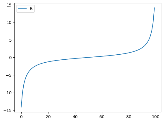

4. Pandas – MultiIndex의 이해

A. 원래 `df`, `s`는 딕셔너리 계열임

- 예시1: df는 dct에서 만들수 있음

dct = {'A': [1,2,3],'B': [2,3,4]}
df = pd.DataFrame(dct)
df

	A	B
0	1	2
1	2	3
2	3	4

df['A']

0    1
1    2
2    3
Name: A, dtype: int64

- 예시2: s도 dct에서 만들수 있음

dct = {'43052': 80, '43053': 90, '43054': 50}
s = pd.Series(dct)
s

43052    80
43053    90
43054    50
dtype: int64

s['43052']

- 예시3: dict의 키로 올수 있는것들?

ref: https://guebin.github.io/PP2023/posts/01_PythonBasic/2023-03-29-4wk-2.html

튜플로 dct를 만든다면?

dct = {('43052',4): 80, ('43053',1): 90, ('43054',2): 50} # (학번,학년)
s = pd.Series(dct)
s

43052  4    80
43053  1    90
43054  2    50
dtype: int64

dct[('43052',4)]

s[('43052',4)]

s.index

MultiIndex([('43052', 4),
            ('43053', 1),
            ('43054', 2)],
           )

B. `.index` 혹은 `.columns`에 `name`이 있는 경우

예시1: index에 이름이 있는 경우 ['id']

dct = {'43052': 80, '43053': 90, '43054': 50}
s = pd.Series(dct)
s

43052    80
43053    90
43054    50
dtype: int64

s.rename_axis(['id'])

id
43052    80
43053    90
43054    50
dtype: int64

s.index, s.rename_axis(['id']).index,

(Index(['43052', '43053', '43054'], dtype='object'),
 Index(['43052', '43053', '43054'], dtype='object', name='id'))

#

예시2: index에 이름이 있는 경우 ['id','year']

dct = {('43052',4): 80, ('43053',1): 90, ('43054',2): 50} # (학번,학년)
s = pd.Series(dct)
s.rename_axis(['id','year'])

id     year
43052  4       80
43053  1       90
43054  2       50
dtype: int64

s.index

MultiIndex([('43052', 4),
            ('43053', 1),
            ('43054', 2)],
           )

s.rename_axis(['id','year']).index

MultiIndex([('43052', 4),
            ('43053', 1),
            ('43054', 2)],
           names=['id', 'year'])

#

dct = {('43052',4): 80, ('43053',1): 90, ('43054',2): 50} # (학번,학년)
s = pd.Series(dct)
s.rename_axis(['id','year'])

id     year
43052  4       80
43053  1       90
43054  2       50
dtype: int64

예시3: 예시2가 데이터프레임이라면 이렇게 보인다

dct = {('43052',4): 80, ('43053',1): 90, ('43054',2): 50} # (학번,학년)
s = pd.Series(dct)
df = pd.DataFrame(s.rename_axis(['id','year']))
df

		0
id	year
43052	4	80
43053	1	90
43054	2	50

df.columns

RangeIndex(start=0, stop=1, step=1)

df.index

MultiIndex([('43052', 4),
            ('43053', 1),
            ('43054', 2)],
           names=['id', 'year'])

#

예시4: 심슨의 역설 – 전체

df=pd.read_csv("https://raw.githubusercontent.com/guebin/DV2022/master/posts/Simpson.csv",index_col=0,header=[0,1])\
.stack().stack().reset_index()\
.rename({'level_0':'department','level_1':'result','level_2':'gender',0:'count'},axis=1).pivot_table(index='gender', columns='result', values='count', aggfunc=sum)
df

/tmp/ipykernel_2417284/2316601964.py:1: FutureWarning: The provided callable <built-in function sum> is currently using DataFrameGroupBy.sum. In a future version of pandas, the provided callable will be used directly. To keep current behavior pass the string "sum" instead.

result	fail	pass
gender
female	1063	772
male	1291	1400

df.index,df.columns

(Index(['female', 'male'], dtype='object', name='gender'),
 Index(['fail', 'pass'], dtype='object', name='result'))

1열과 2열을 더하고 싶다면? 단순히 아래와 같이 하면 된다. (여기에서 gender,result는 각각 index 의 이름, columns의 이름일 뿐이므로 신경쓸 필요 없음)

df['fail']+df['pass']

gender
female    1835
male      2691
dtype: int64

#

예시5: 심슨의 역설 – 학과별

df = pd.read_csv("https://raw.githubusercontent.com/guebin/DV2022/master/posts/Simpson.csv",index_col=0,header=[0,1])\
.stack().stack().reset_index()\
.rename({'level_0':'department','level_1':'result','level_2':'gender',0:'count'},axis=1).pivot_table(index=['gender','department'], columns='result',values='count',aggfunc=sum)
df

/tmp/ipykernel_2417284/2434963071.py:1: FutureWarning: The provided callable <built-in function sum> is currently using DataFrameGroupBy.sum. In a future version of pandas, the provided callable will be used directly. To keep current behavior pass the string "sum" instead.

	result	fail	pass
gender	department
female	A	19	89
	B	7	18
	C	391	202
	D	244	131
	E	299	94
	F	103	238
male	A	314	511
	B	208	352
	C	204	121
	D	279	138
	E	137	54
	F	149	224

df.index, df.columns

(MultiIndex([('female', 'A'),
             ('female', 'B'),
             ('female', 'C'),
             ('female', 'D'),
             ('female', 'E'),
             ('female', 'F'),
             (  'male', 'A'),
             (  'male', 'B'),
             (  'male', 'C'),
             (  'male', 'D'),
             (  'male', 'E'),
             (  'male', 'F')],
            names=['gender', 'department']),
 Index(['fail', 'pass'], dtype='object', name='result'))

학과별 합격률을 알고 싶다면?

df.assign(rate = df['pass']/df.sum(axis=1))

	result	fail	pass	rate
gender	department
female	A	19	89	0.824074
	B	7	18	0.720000
	C	391	202	0.340641
	D	244	131	0.349333
	E	299	94	0.239186
	F	103	238	0.697947
male	A	314	511	0.619394
	B	208	352	0.628571
	C	204	121	0.372308
	D	279	138	0.330935
	E	137	54	0.282723
	F	149	224	0.600536

#

5. Pandas – tidydata

A. tidydata의 개념

- 아래의 자료는 불리하다. (뭐가??)

df = pd.read_csv("https://raw.githubusercontent.com/guebin/DV2022/master/posts/Simpson.csv",index_col=0,header=[0,1])\
.stack().stack().reset_index()\
.rename({'level_0':'department','level_1':'result','level_2':'gender',0:'count'},axis=1).pivot_table(index=['gender','department'], columns='result',values='count',aggfunc=sum)
df

/tmp/ipykernel_2417284/2434963071.py:1: FutureWarning: The provided callable <built-in function sum> is currently using DataFrameGroupBy.sum. In a future version of pandas, the provided callable will be used directly. To keep current behavior pass the string "sum" instead.

	result	fail	pass
gender	department
female	A	19	89
	B	7	18
	C	391	202
	D	244	131
	E	299	94
	F	103	238
male	A	314	511
	B	208	352
	C	204	121
	D	279	138
	E	137	54
	F	149	224

- 가정1: 만약에 A학과에 해당하는 결과만 뽑고 싶다면? –> departmet가 column으로 있어야함..

- 가정2: 이 데이터를 바탕으로 합격한사람만 bar plot을 그리고 싶다면? –> department, gender, pass 가 column으로 있어야함..

tidydata = df['pass'].reset_index()
#---# 
fig = ggplot(tidydata)
col = geom_col(aes(x='department',y='pass',fill='gender'),position='dodge')
fig + col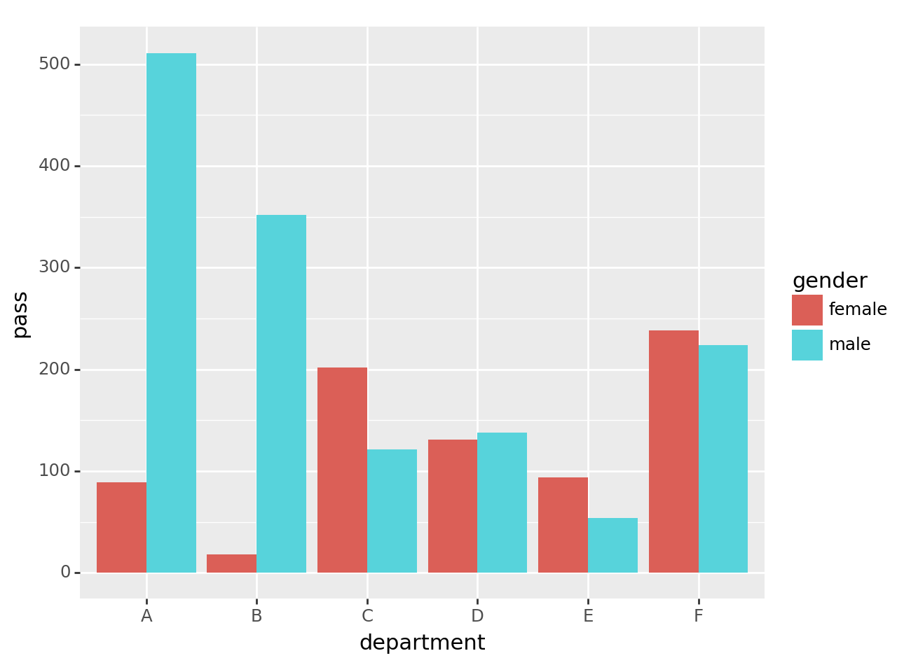

- tidydata 정의: https://r4ds.had.co.nz/tidy-data.html

Each variable must have its own column.
Each observation must have its own row.
Each value must have its own cell.

B. tidydata가 아닌 예시

예시1 – MultiIndex 구조를 가지면 무조건 tidydata가 아니다.

df = pd.read_csv("https://raw.githubusercontent.com/guebin/DV2022/master/posts/Simpson.csv",index_col=0,header=[0,1])\
.stack().stack().reset_index()\
.rename({'level_0':'department','level_1':'result','level_2':'gender',0:'count'},axis=1).pivot_table(index=['gender','department'], columns='result',values='count',aggfunc=sum)
df

/tmp/ipykernel_2417284/2434963071.py:1: FutureWarning: The provided callable <built-in function sum> is currently using DataFrameGroupBy.sum. In a future version of pandas, the provided callable will be used directly. To keep current behavior pass the string "sum" instead.

	result	fail	pass
gender	department
female	A	19	89
	B	7	18
	C	391	202
	D	244	131
	E	299	94
	F	103	238
male	A	314	511
	B	208	352
	C	204	121
	D	279	138
	E	137	54
	F	149	224

이건 tidydata가 아니고

tidydata = df.stack().reset_index().rename({0:'applicant_count'},axis=1)
tidydata

	gender	department	result	applicant_count
0	female	A	fail	19
1	female	A	pass	89
2	female	B	fail	7
3	female	B	pass	18
4	female	C	fail	391
5	female	C	pass	202
6	female	D	fail	244
7	female	D	pass	131
8	female	E	fail	299
9	female	E	pass	94
10	female	F	fail	103
11	female	F	pass	238
12	male	A	fail	314
13	male	A	pass	511
14	male	B	fail	208
15	male	B	pass	352
16	male	C	fail	204
17	male	C	pass	121
18	male	D	fail	279
19	male	D	pass	138
20	male	E	fail	137
21	male	E	pass	54
22	male	F	fail	149
23	male	F	pass	224

이것이 tidydata

- 구분하는 방법1: 직관에 의한 설명

query쓰기 불편: 남성지원자만 뽑고 싶다면?, 학과A만 뽑고싶다면? 탈락한지원자만 뽑고싶다면? 학과A에서 탈락한 지원자만 뽑고싶다면??
시각화하기 불편:
하여튼 다루기 불편해..

- 구분하는 방법2: 정의에 의한 설명

df는 원칙 1에 위배된다. (왜냐하면 gender, department,result,applicant_count에 해당하는 변수는 하나의 컬럼을 차지하지 못함)
df는 원칙 2에 위배된다. (왜냐하면 하나의 행에 2개의 applicant_count observation이 존재함)

#

예시2 – 아래의 자료는 tidydata가 아니다.

df=pd.read_csv("https://raw.githubusercontent.com/guebin/DV2022/master/posts/Simpson.csv",index_col=0,header=[0,1])\
.stack().stack().reset_index()\
.rename({'level_0':'department','level_1':'result','level_2':'gender',0:'count'},axis=1).pivot_table(index='gender', columns='result', values='count', aggfunc=sum)\
.assign(pass_fail = lambda df: list(map(lambda x,y: (y,x),df['fail'],df['pass']))).drop(['fail','pass'],axis=1).reset_index()
df

/tmp/ipykernel_2278789/2865855793.py:1: FutureWarning: The provided callable <built-in function sum> is currently using DataFrameGroupBy.sum. In a future version of pandas, the provided callable will be used directly. To keep current behavior pass the string "sum" instead.

result	gender	pass_fail
0	female	(772, 1063)
1	male	(1400, 1291)

이 df는 원칙 3에 위배된다.

#

# 예시3 – wide df

df=pd.read_csv('https://raw.githubusercontent.com/guebin/2021DV/master/_notebooks/phone.csv')
df

	Date	Samsung	Apple	Huawei	Xiaomi	Oppo	Mobicel	Motorola	LG	Others	Realme	Google	Nokia	Lenovo	OnePlus	Sony	Asus
0	2019-10	461	324	136	109	76	81	43	37	135	28	39	14	22	17	20	17
1	2019-11	461	358	167	141	86	61	29	36	141	27	29	20	23	10	19	27
2	2019-12	426	383	143	105	53	45	51	48	129	30	20	26	28	18	18	19
3	2020-01	677	494	212	187	110	79	65	49	158	23	13	19	19	22	27	22
4	2020-02	593	520	217	195	112	67	62	71	157	25	18	16	24	18	23	20
5	2020-03	637	537	246	187	92	66	59	67	145	21	16	24	18	31	22	14
6	2020-04	647	583	222	154	98	59	48	64	113	20	23	25	19	19	23	21
7	2020-05	629	518	192	176	91	87	50	66	150	43	27	15	18	19	19	13
8	2020-06	663	552	209	185	93	69	54	60	140	39	16	16	17	29	25	16
9	2020-07	599	471	214	193	89	78	65	59	130	40	27	25	21	18	18	12
10	2020-08	615	567	204	182	105	82	62	42	129	47	16	23	21	27	23	20
11	2020-09	621	481	230	220	102	88	56	49	143	54	14	15	17	15	19	15
12	2020-10	637	555	232	203	90	52	63	49	140	33	17	20	22	9	22	21

이건 tidydata 가 아니고

tidydata = df.melt(id_vars='Date').assign(Date = lambda _df: _df.Date.apply(pd.to_datetime))
tidydata

	Date	variable	value
0	2019-10-01	Samsung	461
1	2019-11-01	Samsung	461
2	2019-12-01	Samsung	426
3	2020-01-01	Samsung	677
4	2020-02-01	Samsung	593
...	...	...	...
203	2020-06-01	Asus	16
204	2020-07-01	Asus	12
205	2020-08-01	Asus	20
206	2020-09-01	Asus	15
207	2020-10-01	Asus	21

208 rows × 3 columns

이건 tidydata 이다.

- df를 가지고 아래와 같은 그림을 그릴 수 있겠어?

fig = ggplot(tidydata)
line = geom_line(aes(x='Date',y='value',color='variable'))
fig + line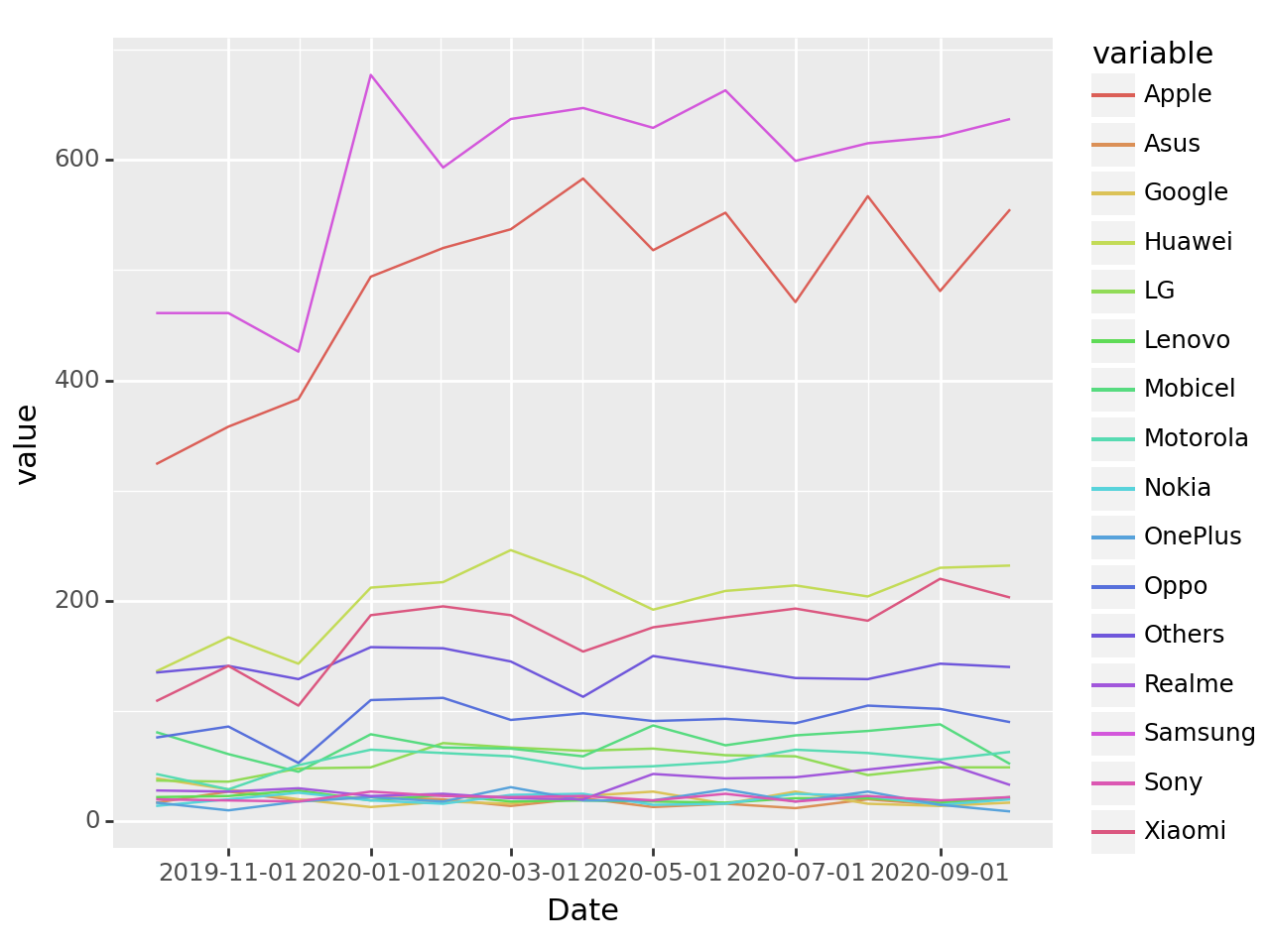

6. Pandas – `melt`/`stack`

A. `reset_index()`

중첩구조를 가지는 series일 경우 .reset_index()를 사용하면 쉽게 tidydata를 얻을 수 있다.

- 예시1

dct = {'43052': 80, '43053': 90, '43054': 50}
s = pd.Series(dct)
s

43052    80
43053    90
43054    50
dtype: int64

s.reset_index()

	index	0
0	43052	80
1	43053	90
2	43054	50

- 예시2

dct = {('43052',4): 80, ('43053',1): 90, ('43054',2): 50} # (학번,학년)
s = pd.Series(dct)
s

43052  4    80
43053  1    90
43054  2    50
dtype: int64

s.reset_index()

	level_0	level_1	0
0	43052	4	80
1	43053	1	90
2	43054	2	50

- 예시3

df=pd.read_csv("https://raw.githubusercontent.com/guebin/DV2022/master/posts/Simpson.csv",index_col=0,header=[0,1]).stack().stack()
df

A  fail  male      314
         female     19
   pass  male      511
         female     89
B  fail  male      208
         female      7
   pass  male      352
         female     18
C  fail  male      204
         female    391
   pass  male      121
         female    202
D  fail  male      279
         female    244
   pass  male      138
         female    131
E  fail  male      137
         female    299
   pass  male       54
         female     94
F  fail  male      149
         female    103
   pass  male      224
         female    238
dtype: int64

df.reset_index()

	level_0	level_1	level_2	0
0	A	fail	male	314
1	A	fail	female	19
2	A	pass	male	511
3	A	pass	female	89
4	B	fail	male	208
5	B	fail	female	7
6	B	pass	male	352
7	B	pass	female	18
8	C	fail	male	204
9	C	fail	female	391
10	C	pass	male	121
11	C	pass	female	202
12	D	fail	male	279
13	D	fail	female	244
14	D	pass	male	138
15	D	pass	female	131
16	E	fail	male	137
17	E	fail	female	299
18	E	pass	male	54
19	E	pass	female	94
20	F	fail	male	149
21	F	fail	female	103
22	F	pass	male	224
23	F	pass	female	238

- 예시4 – .reset_index() 는 말그대로 index를 reset 하는 명령어, 꼭 pd.Series에만 쓰는건 아니다.

df=pd.read_csv("https://raw.githubusercontent.com/guebin/DV2022/master/posts/Simpson.csv",index_col=0,header=[0,1]).stack()
df

		male	female
A	fail	314	19
A	pass	511	89
B	fail	208	7
B	pass	352	18
C	fail	204	391
C	pass	121	202
D	fail	279	244
D	pass	138	131
E	fail	137	299
E	pass	54	94
F	fail	149	103
F	pass	224	238

df.reset_index()

	level_0	level_1	male	female
0	A	fail	314	19
1	A	pass	511	89
2	B	fail	208	7
3	B	pass	352	18
4	C	fail	204	391
5	C	pass	121	202
6	D	fail	279	244
7	D	pass	138	131
8	E	fail	137	299
9	E	pass	54	94
10	F	fail	149	103
11	F	pass	224	238

B. `melt()`

# 예시1: 아래의 자료를 tidydata로 만들라.

df = pd.read_csv('https://raw.githubusercontent.com/guebin/2021DV/master/_notebooks/phone.csv')
df

	Date	Samsung	Apple	Huawei	Xiaomi	Oppo	Mobicel	Motorola	LG	Others	Realme	Google	Nokia	Lenovo	OnePlus	Sony	Asus
0	2019-10	461	324	136	109	76	81	43	37	135	28	39	14	22	17	20	17
1	2019-11	461	358	167	141	86	61	29	36	141	27	29	20	23	10	19	27
2	2019-12	426	383	143	105	53	45	51	48	129	30	20	26	28	18	18	19
3	2020-01	677	494	212	187	110	79	65	49	158	23	13	19	19	22	27	22
4	2020-02	593	520	217	195	112	67	62	71	157	25	18	16	24	18	23	20
5	2020-03	637	537	246	187	92	66	59	67	145	21	16	24	18	31	22	14
6	2020-04	647	583	222	154	98	59	48	64	113	20	23	25	19	19	23	21
7	2020-05	629	518	192	176	91	87	50	66	150	43	27	15	18	19	19	13
8	2020-06	663	552	209	185	93	69	54	60	140	39	16	16	17	29	25	16
9	2020-07	599	471	214	193	89	78	65	59	130	40	27	25	21	18	18	12
10	2020-08	615	567	204	182	105	82	62	42	129	47	16	23	21	27	23	20
11	2020-09	621	481	230	220	102	88	56	49	143	54	14	15	17	15	19	15
12	2020-10	637	555	232	203	90	52	63	49	140	33	17	20	22	9	22	21

(풀이1) .melt() – 실패

df.melt()

	variable	value
0	Date	2019-10
1	Date	2019-11
2	Date	2019-12
3	Date	2020-01
4	Date	2020-02
...	...	...
216	Asus	16
217	Asus	12
218	Asus	20
219	Asus	15
220	Asus	21

221 rows × 2 columns

(풀이2) .melt(id_vars=) – 성공

df.melt(id_vars='Date')

	Date	variable	value
0	2019-10	Samsung	461
1	2019-11	Samsung	461
2	2019-12	Samsung	426
3	2020-01	Samsung	677
4	2020-02	Samsung	593
...	...	...	...
203	2020-06	Asus	16
204	2020-07	Asus	12
205	2020-08	Asus	20
206	2020-09	Asus	15
207	2020-10	Asus	21

208 rows × 3 columns

#

C. `stack()` + `reset_index()`

제 최애테크닉: DataFrame을 MultiIndex를 가지는 Series로 “일부러” 변환하고 reset_index()를 시킴

# 예시1: 아래의 자료를 tidydata로 만들라.

df = pd.read_csv('https://raw.githubusercontent.com/guebin/2021DV/master/_notebooks/phone.csv')
df

	Date	Samsung	Apple	Huawei	Xiaomi	Oppo	Mobicel	Motorola	LG	Others	Realme	Google	Nokia	Lenovo	OnePlus	Sony	Asus
0	2019-10	461	324	136	109	76	81	43	37	135	28	39	14	22	17	20	17
1	2019-11	461	358	167	141	86	61	29	36	141	27	29	20	23	10	19	27
2	2019-12	426	383	143	105	53	45	51	48	129	30	20	26	28	18	18	19
3	2020-01	677	494	212	187	110	79	65	49	158	23	13	19	19	22	27	22
4	2020-02	593	520	217	195	112	67	62	71	157	25	18	16	24	18	23	20
5	2020-03	637	537	246	187	92	66	59	67	145	21	16	24	18	31	22	14
6	2020-04	647	583	222	154	98	59	48	64	113	20	23	25	19	19	23	21
7	2020-05	629	518	192	176	91	87	50	66	150	43	27	15	18	19	19	13
8	2020-06	663	552	209	185	93	69	54	60	140	39	16	16	17	29	25	16
9	2020-07	599	471	214	193	89	78	65	59	130	40	27	25	21	18	18	12
10	2020-08	615	567	204	182	105	82	62	42	129	47	16	23	21	27	23	20
11	2020-09	621	481	230	220	102	88	56	49	143	54	14	15	17	15	19	15
12	2020-10	637	555	232	203	90	52	63	49	140	33	17	20	22	9	22	21

df.set_index('Date').stack().reset_index()

	Date	level_1	0
0	2019-10	Samsung	461
1	2019-10	Apple	324
2	2019-10	Huawei	136
3	2019-10	Xiaomi	109
4	2019-10	Oppo	76
...	...	...	...
203	2020-10	Nokia	20
204	2020-10	Lenovo	22
205	2020-10	OnePlus	9
206	2020-10	Sony	22
207	2020-10	Asus	21

208 rows × 3 columns

#

# 예시2: 아래의 자료를 tidydata로 만들어라.

df = pd.read_csv("https://raw.githubusercontent.com/guebin/DV2022/master/posts/Simpson.csv",index_col=0,header=[0,1])
df

	male		female
	fail	pass	fail	pass
A	314	511	19	89
B	208	352	7	18
C	204	121	391	202
D	279	138	244	131
E	137	54	299	94
F	149	224	103	238

df.stack().stack().reset_index()

	level_0	level_1	level_2	0
0	A	fail	male	314
1	A	fail	female	19
2	A	pass	male	511
3	A	pass	female	89
4	B	fail	male	208
5	B	fail	female	7
6	B	pass	male	352
7	B	pass	female	18
8	C	fail	male	204
9	C	fail	female	391
10	C	pass	male	121
11	C	pass	female	202
12	D	fail	male	279
13	D	fail	female	244
14	D	pass	male	138
15	D	pass	female	131
16	E	fail	male	137
17	E	fail	female	299
18	E	pass	male	54
19	E	pass	female	94
20	F	fail	male	149
21	F	fail	female	103
22	F	pass	male	224
23	F	pass	female	238

#

D. `unstack() + reset_index()`

# 예시1 – .stack()과 .unstack()은 반대연산

df=pd.read_csv('https://raw.githubusercontent.com/PacktPublishing/Pandas-Cookbook/master/data/flights.csv')\
.groupby(["AIRLINE","WEEKDAY"]).agg({"CANCELLED":[np.mean,"count"],"DIVERTED":[np.mean,"count"]})
df

/tmp/ipykernel_2417284/3693914824.py:2: FutureWarning: The provided callable <function mean at 0x7fbb9032c310> is currently using SeriesGroupBy.mean. In a future version of pandas, the provided callable will be used directly. To keep current behavior pass the string "mean" instead.
/tmp/ipykernel_2417284/3693914824.py:2: FutureWarning: The provided callable <function mean at 0x7fbb9032c310> is currently using SeriesGroupBy.mean. In a future version of pandas, the provided callable will be used directly. To keep current behavior pass the string "mean" instead.

		CANCELLED		DIVERTED
		mean	count	mean	count
AIRLINE	WEEKDAY
AA	1	0.032106	1277	0.004699	1277
	2	0.007341	1226	0.001631	1226
	3	0.011949	1339	0.001494	1339
	4	0.015004	1333	0.003751	1333
	5	0.014151	1272	0.000786	1272
...	...	...	...	...	...
WN	3	0.014118	1275	0.001569	1275
	4	0.007911	1264	0.003165	1264
	5	0.005828	1201	0.000000	1201
	6	0.010132	987	0.003040	987
	7	0.006066	1154	0.002600	1154

98 rows × 4 columns

df.stack().unstack()

		CANCELLED		DIVERTED
		mean	count	mean	count
AIRLINE	WEEKDAY
AA	1	0.032106	1277.0	0.004699	1277.0
	2	0.007341	1226.0	0.001631	1226.0
	3	0.011949	1339.0	0.001494	1339.0
	4	0.015004	1333.0	0.003751	1333.0
	5	0.014151	1272.0	0.000786	1272.0
...	...	...	...	...	...
WN	3	0.014118	1275.0	0.001569	1275.0
	4	0.007911	1264.0	0.003165	1264.0
	5	0.005828	1201.0	0.000000	1201.0
	6	0.010132	987.0	0.003040	987.0
	7	0.006066	1154.0	0.002600	1154.0

98 rows × 4 columns

#

# 예시2 – 아래의 자료를 tidydata로 만들라.

df=pd.read_csv('https://raw.githubusercontent.com/PacktPublishing/Pandas-Cookbook/master/data/flights.csv')\
.groupby(["AIRLINE","WEEKDAY"]).agg({"CANCELLED":[np.mean,"count"],"DIVERTED":[np.mean,"count"]})
df

/tmp/ipykernel_2417284/3693914824.py:2: FutureWarning: The provided callable <function mean at 0x7fbb9032c310> is currently using SeriesGroupBy.mean. In a future version of pandas, the provided callable will be used directly. To keep current behavior pass the string "mean" instead.
/tmp/ipykernel_2417284/3693914824.py:2: FutureWarning: The provided callable <function mean at 0x7fbb9032c310> is currently using SeriesGroupBy.mean. In a future version of pandas, the provided callable will be used directly. To keep current behavior pass the string "mean" instead.

		CANCELLED		DIVERTED
		mean	count	mean	count
AIRLINE	WEEKDAY
AA	1	0.032106	1277	0.004699	1277
	2	0.007341	1226	0.001631	1226
	3	0.011949	1339	0.001494	1339
	4	0.015004	1333	0.003751	1333
	5	0.014151	1272	0.000786	1272
...	...	...	...	...	...
WN	3	0.014118	1275	0.001569	1275
	4	0.007911	1264	0.003165	1264
	5	0.005828	1201	0.000000	1201
	6	0.010132	987	0.003040	987
	7	0.006066	1154	0.002600	1154

98 rows × 4 columns

(풀이1) – stack 2번

df.stack().stack().reset_index()

	AIRLINE	WEEKDAY	level_2	level_3	0
0	AA	1	mean	CANCELLED	0.032106
1	AA	1	mean	DIVERTED	0.004699
2	AA	1	count	CANCELLED	1277.000000
3	AA	1	count	DIVERTED	1277.000000
4	AA	2	mean	CANCELLED	0.007341
...	...	...	...	...	...
387	WN	6	count	DIVERTED	987.000000
388	WN	7	mean	CANCELLED	0.006066
389	WN	7	mean	DIVERTED	0.002600
390	WN	7	count	CANCELLED	1154.000000
391	WN	7	count	DIVERTED	1154.000000

392 rows × 5 columns

(풀이2) – unstack 2번

df.unstack().unstack().reset_index()

	level_0	level_1	WEEKDAY	AIRLINE	0
0	CANCELLED	mean	1	AA	0.032106
1	CANCELLED	mean	1	AS	0.000000
2	CANCELLED	mean	1	B6	0.000000
3	CANCELLED	mean	1	DL	0.006068
4	CANCELLED	mean	1	EV	0.034130
...	...	...	...	...	...
387	DIVERTED	count	7	OO	924.000000
388	DIVERTED	count	7	UA	1038.000000
389	DIVERTED	count	7	US	263.000000
390	DIVERTED	count	7	VX	135.000000
391	DIVERTED	count	7	WN	1154.000000

392 rows × 5 columns

예시3 – 아래의 자료를 tidydata로 만들어라.

df=pd.read_csv("https://raw.githubusercontent.com/guebin/DV2022/master/posts/Simpson.csv",index_col=0,header=[0,1])
df

	male		female
	fail	pass	fail	pass
A	314	511	19	89
B	208	352	7	18
C	204	121	391	202
D	279	138	244	131
E	137	54	299	94
F	149	224	103	238

(풀이1) – stack 2번

df.stack().stack().reset_index()

	level_0	level_1	level_2	0
0	A	fail	male	314
1	A	fail	female	19
2	A	pass	male	511
3	A	pass	female	89
4	B	fail	male	208
5	B	fail	female	7
6	B	pass	male	352
7	B	pass	female	18
8	C	fail	male	204
9	C	fail	female	391
10	C	pass	male	121
11	C	pass	female	202
12	D	fail	male	279
13	D	fail	female	244
14	D	pass	male	138
15	D	pass	female	131
16	E	fail	male	137
17	E	fail	female	299
18	E	pass	male	54
19	E	pass	female	94
20	F	fail	male	149
21	F	fail	female	103
22	F	pass	male	224
23	F	pass	female	238

(풀이2) – unstack 1번

df.unstack().reset_index()

	level_0	level_1	level_2	0
0	male	fail	A	314
1	male	fail	B	208
2	male	fail	C	204
3	male	fail	D	279
4	male	fail	E	137
5	male	fail	F	149
6	male	pass	A	511
7	male	pass	B	352
8	male	pass	C	121
9	male	pass	D	138
10	male	pass	E	54
11	male	pass	F	224
12	female	fail	A	19
13	female	fail	B	7
14	female	fail	C	391
15	female	fail	D	244
16	female	fail	E	299
17	female	fail	F	103
18	female	pass	A	89
19	female	pass	B	18
20	female	pass	C	202
21	female	pass	D	131
22	female	pass	E	94
23	female	pass	F	238

7. HW

아래의 자료를 tidydata로 변환하라.

s = pd.Series({
    ('female','A'):0.5,
    ('female','B'):0.2,
    ('male','A'):0.3,
    ('male','B'):0.7
})
s

female  A    0.5
        B    0.2
male    A    0.3
        B    0.7
dtype: float64

# 출력결과는 아래와 같아야 한다.

	level_0	level_1	0
0	female	A	0.5
1	female	B	0.2
2	male	A	0.3
3	male	B	0.7

1. 강의영상

2. Imports

3. Pandas – lambda df:의 활용

A. lambda df: with indexer

B. lambda df: with assign

4. Pandas – MultiIndex의 이해

A. 원래 df, s는 딕셔너리 계열임

B. .index 혹은 .columns에 name이 있는 경우

5. Pandas – tidydata

A. tidydata의 개념

B. tidydata가 아닌 예시

6. Pandas – melt/stack

A. reset_index()

B. melt()

C. stack() + reset_index()

D. unstack() + reset_index()

7. HW

3. Pandas – `lambda df:`의 활용

A. `lambda df:` with indexer

B. `lambda df:` with assign

A. 원래 `df`, `s`는 딕셔너리 계열임

B. `.index` 혹은 `.columns`에 `name`이 있는 경우

6. Pandas – `melt`/`stack`

A. `reset_index()`

B. `melt()`

C. `stack()` + `reset_index()`

D. `unstack() + reset_index()`