import torch
import torchvision
import matplotlib.pyplot as plt06wk-2: (신경망) – 다항분류, FashionMNIST
![]()
1. 강의영상
2. Imports
plt.rcParams['figure.figsize'] = (4.5, 3.0)3. 다항분류
A. 이항분류와 BCEWithLogitsLoss
- 데이터
train_dataset = torchvision.datasets.MNIST(root='./data', train=True, download=True)
to_tensor = torchvision.transforms.ToTensor()
X0_train = torch.stack([to_tensor(Xi) for Xi, yi in train_dataset if yi==0])
X1_train = torch.stack([to_tensor(Xi) for Xi, yi in train_dataset if yi==1])
X = torch.concat([X0_train,X1_train],axis=0).reshape(-1,784)
y = torch.tensor([0.0]*len(X0_train) + [1.0]*len(X1_train)).reshape(-1,1)
- 예전에 적합했던 코드에서 sig를 분리한것
torch.manual_seed(43052)
net = torch.nn.Sequential(
    torch.nn.Linear(784,32),
    torch.nn.ReLU(),
    torch.nn.Linear(32,1),
)
sig = torch.nn.Sigmoid()
loss_fn = torch.nn.BCELoss()
optimizr = torch.optim.Adam(net.parameters())
#---#
for epoc in range(1,31):
    #1
    netout = net(X)
    yhat = sig(netout)
    #2
    loss = loss_fn(yhat,y)
    #3
    loss.backward()
    #4
    optimizr.step()
    optimizr.zero_grad()
# netout(=logits) 의 특징
- \(netout >0 \Leftrightarrow sig(netout) > 0.5\)
- \(netout <0 \Leftrightarrow sig(netout) < 0.5\)
((net(X)>0) ==y).float().mean()tensor(0.9956)- 아래의 코드는 위의 코드와 같은 코드임
torch.manual_seed(43052)
net = torch.nn.Sequential(
    torch.nn.Linear(784,32),
    torch.nn.ReLU(),
    torch.nn.Linear(32,1),
)
loss_fn = torch.nn.BCEWithLogitsLoss()
optimizr = torch.optim.Adam(net.parameters())
#---#
for epoc in range(1,31):
    #1
    netout = net(X)
    #2
    loss = loss_fn(netout,y)
    #3
    loss.backward()
    #4
    optimizr.step()
    optimizr.zero_grad()
B. 범주형자료의 변환
- 범주형자료를 숫자로 어떻게 바꿀까?
- 실패 / 성공 \(\to\) 0 / 1
- 숫자0그림 / 숫자1그림 \(\to\) 0 / 1
- 강아지그림 / 고양이그림 \(\to\) 0 / 1
- 강아지그림 / 고양이그림 / 토끼그림 \(\to\) 0 / 1 / 2 ?????
- 주입식교육: 강아지그림/고양이그림/토끼그림일 경우 숫자화시키는 방법
- 잘못된방식: 강아지그림 = 0, 고양이그림 = 1, 토끼그림 = 2
- 올바른방식: 강아지그림 = [1,0,0], 고양이그림 = [0,1,0], 토끼그림 = [0,0,1] ### <– 이런방식을 원핫인코딩이라함
- 왜?
- 설명1: 강아지그림, 고양이그림, 토끼그림은 서열측도가 아니라 명목척도임. 그래서 범주를 0,1,2 로 숫자화하면 평균등의 의미가 없음 (사회조사분석사 2급 스타일)
- 설명2: 범주형은 원핫인코딩으로 해야함 (“30일만에 끝내는 실전머신러닝” 이런 책에 나오는 스타일)
- 설명3: 동전을 한번 던져서 나오는 결과는 \(n=1\)인 이항분포를 따름. 주사위 한번 던져서 나오는 눈금의 숫자는 \(n=1\)인 다항분포를 따름. \(n=1\)인 이항분포의 실현값은 0,1 이고, \(n=1\)인 다항분포의 실현값은 [1,0,0], [0,1,0], [0,0,1] 이므로 당연히 \(y_i\) 는 [1,0,0], [0,1,0], [0,0,1] 중 하나의 형태를 가진다고 가정하는게 바람직함 (이 설명이 이 중에서 가장 정확한 설명임)
C. 실습: 3개의 클래스를 구분
- 데이터준비
train_dataset = torchvision.datasets.MNIST(root='./data', train=True, download=True)
to_tensor = torchvision.transforms.ToTensor()
X0 = torch.stack([to_tensor(Xi) for Xi, yi in train_dataset if yi==0])
X1 = torch.stack([to_tensor(Xi) for Xi, yi in train_dataset if yi==1])
X2 = torch.stack([to_tensor(Xi) for Xi, yi in train_dataset if yi==2])
X = torch.concat([X0,X1,X2]).reshape(-1,1*28*28)
y = torch.tensor([0]*len(X0) + [1]*len(X1)+ [2]*len(X2)).reshape(-1,1).float()
y = torch.nn.functional.one_hot(y.reshape(-1).long()).float()
ytensor([[1., 0., 0.],
[1., 0., 0.],
[1., 0., 0.],
...,
[0., 0., 1.],
[0., 0., 1.],
[0., 0., 1.]])- 적합
net = torch.nn.Sequential(
    torch.nn.Linear(784,32),
    torch.nn.ReLU(),
    torch.nn.Linear(32,3),
)
loss_fn = torch.nn.CrossEntropyLoss() # 의미상 CEWithLogitsLoss
optimizr = torch.optim.Adam(net.parameters())
for epoc in range(1,31):
    #1
    netout = net(X) # netout: (n,3)
    #2
    loss = loss_fn(netout,y)
    #3
    loss.backward()
    #4
    optimizr.step()
optimizr.zero_grad()(netout.argmax(axis=1) == y.argmax(axis=1)).float().mean()tensor(0.9669)D. 결론 – 외우세여
- 파이토치버전 // 코딩용
| 분류 | netout의 의미 | 손실함수 |
|---|---|---|
| 이항분류 | prob | BCELoss |
| 이항분류 | logit | BCEWithLogitsLoss |
| 다항분류 | probs | NA |
| 다항분류 | logits | CrossEntropyLoss |
CrossEntropyLoss이거 이름이 완전 마음에 안들어요..CEWithLogitsLoss라고 하는게 더 좋을 것 같습니다.
- 일반적개념 // 이론용
| 분류 | 오차항의가정 | 마지막활성화함수 | 손실함수 |
|---|---|---|---|
| 이항분류 | 이항분포 | sigmoid1 | Binary Cross Entropy |
| 다항분류 | 다항분포 | softmax2 | Cross Entropy |
1 prob=sig(logit)
2 probs=soft(logits)
- 참고 (sigmoid, softmax 계산과정비교)
- \(prob = \text{sig}(logit) =\frac{\exp(logit)}{1+\exp(logit)}\)
- \(probs= \text{softmax}\left(\begin{bmatrix} logit_1 \\ logit_2 \\ logit_3\end{bmatrix}\right) =\begin{bmatrix} \frac{\exp(logit_1)}{\exp(logit_1)+\exp(logit_2)+\exp(logit_3)} \\ \frac{\exp(logit_2)}{\exp(logit_1)+\exp(logit_2)+\exp(logit_3)} \\ \frac{\exp(logit_3)}{\exp(logit_1)+\exp(logit_2)+\exp(logit_3)} \end{bmatrix}\)
4. FashionMNIST
A. 데이터
https://arxiv.org/abs/1708.07747 (Xiao, Rasul, and Vollgraf 2017)
Xiao, Han, Kashif Rasul, and Roland Vollgraf. 2017. “Fashion-Mnist: A Novel Image Dataset for Benchmarking Machine Learning Algorithms.” arXiv Preprint arXiv:1708.07747.
train_dataset = torchvision.datasets.FashionMNIST(root='./data', train=True, download=True)
test_dataset = torchvision.datasets.FashionMNIST(root='./data', train=False, download=True)
to_tensor = torchvision.transforms.ToTensor()
X = torch.stack([to_tensor(img) for img, lbl in train_dataset])
y = torch.tensor([lbl for img, lbl in train_dataset])
y = torch.nn.functional.one_hot(y).float()
XX = torch.stack([to_tensor(img) for img, lbl in test_dataset])
yy = torch.tensor([lbl for img, lbl in test_dataset])
yy = torch.nn.functional.one_hot(yy).float()
obs_idx = 301
plt.imshow(X[obs_idx,0,:,:],cmap="gray")
plt.title(torchvision.datasets.FashionMNIST.classes[y[obs_idx,:].argmax().item()]);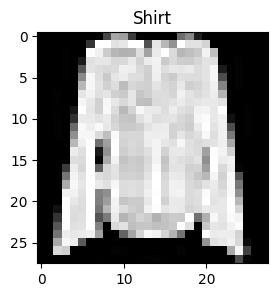
B. 간단한 신경망
- Step1: 데이터정리
ds_train = torch.utils.data.TensorDataset(X,y)
dl_train = torch.utils.data.DataLoader(ds_train,batch_size=256,shuffle=True)
ds_test = torch.utils.data.TensorDataset(XX,yy)
dl_test = torch.utils.data.DataLoader(ds_test,batch_size=256)
- Step2: 학습에 필요한 준비 (모델링)
torch.manual_seed(43052)
net = torch.nn.Sequential(
    torch.nn.Flatten(),
    torch.nn.Linear(784,32),
    torch.nn.ReLU(),
    torch.nn.Linear(32,10)
).to("cuda:0")
loss_fn = torch.nn.CrossEntropyLoss()
optimizr = torch.optim.Adam(net.parameters())
#---#
- Step3: 적합
for epoc in range(1,31):
    net.train()
    #---에폭시작---#
    for Xm,ym in dl_train:
        Xm = Xm.to("cuda:0")
        ym = ym.to("cuda:0")
        # 1
        netout = net(Xm)
        # 2
        loss = loss_fn(netout,ym)
        # 3
        loss.backward()
        # 4
        optimizr.step()
        optimizr.zero_grad()
    #---에폭끝---#
    if epoc % 5 == 0:
        net.eval()
        s =0
        for Xm,ym in dl_train:
            Xm = Xm.to("cuda:0")
            ym = ym.to("cuda:0")
            logits = net(Xm).data
            s = s+ (logits.argmax(axis=1) == ym.argmax(axis=1)).float().sum()
        acc = s / len(X)
        print(f"# of epochs = {epoc},train_acc = {acc:.4f}")
# of epochs = 5,train_acc = 0.8588
# of epochs = 10,train_acc = 0.8659
# of epochs = 15,train_acc = 0.8779
# of epochs = 20,train_acc = 0.8830
# of epochs = 25,train_acc = 0.8857
# of epochs = 30,train_acc = 0.8875- Step4: 적합결과 시각화 및 분석
net.eval()
s =0
for Xm,ym in dl_test:
    Xm = Xm.to("cuda:0")
    ym = ym.to("cuda:0")
    logits = net(Xm).data
    s = s+ (logits.argmax(axis=1) == ym.argmax(axis=1)).float().sum()
acc = s / len(XX)
print(f"test_acc = {acc:.4f}")
test_acc = 0.8639C. 약간 더 복잡한 신경망
torch.manual_seed(43052)
net = torch.nn.Sequential(
    torch.nn.Flatten(),
    torch.nn.Linear(784,256),
    torch.nn.ReLU(),
    torch.nn.Linear(256,10)
).to("cuda:0")
loss_fn = torch.nn.CrossEntropyLoss()
optimizr = torch.optim.Adam(net.parameters())
#---#
for epoc in range(1,31):
net.train()
#---에폭시작---#
for Xm,ym in dl_train:
Xm = Xm.to("cuda:0")
ym = ym.to("cuda:0")
# 1
netout = net(Xm)
# 2
loss = loss_fn(netout,ym)
# 3
loss.backward()
# 4
optimizr.step()
optimizr.zero_grad()
#---에폭끝---#
if epoc % 5 == 0:
net.eval()
s =0
for Xm,ym in dl_train:
Xm = Xm.to("cuda:0")
ym = ym.to("cuda:0")
logits = net(Xm).data
s = s+ (logits.argmax(axis=1) == ym.argmax(axis=1)).float().sum()
acc = s / len(X)
print(f"# of epochs = {epoc},train_acc = {acc:.4f}") # of epochs = 5,train_acc = 0.8831
# of epochs = 10,train_acc = 0.9028
# of epochs = 15,train_acc = 0.9183
# of epochs = 20,train_acc = 0.9281
# of epochs = 25,train_acc = 0.9331
# of epochs = 30,train_acc = 0.9332net.eval()
s =0
for Xm,ym in dl_test:
Xm = Xm.to("cuda:0")
ym = ym.to("cuda:0")
logits = net(Xm).data
s = s+ (logits.argmax(axis=1) == ym.argmax(axis=1)).float().sum()
acc = s / len(XX)
print(f"test_acc = {acc:.4f}") test_acc = 0.8833D. 발악
- 노드를 많이..
torch.manual_seed(43052)
net = torch.nn.Sequential(
    torch.nn.Flatten(),
    torch.nn.Linear(784,4096),
    torch.nn.Dropout(0.5),
    torch.nn.ReLU(),
    torch.nn.Linear(4096,10)
).to("cuda:0")
loss_fn = torch.nn.CrossEntropyLoss()
optimizr = torch.optim.Adam(net.parameters())
#---#
for epoc in range(1,31):
net.train()
#---에폭시작---#
for Xm,ym in dl_train:
Xm = Xm.to("cuda:0")
ym = ym.to("cuda:0")
# 1
netout = net(Xm)
# 2
loss = loss_fn(netout,ym)
# 3
loss.backward()
# 4
optimizr.step()
optimizr.zero_grad()
#---에폭끝---#
if epoc % 5 == 0:
net.eval()
s =0
for Xm,ym in dl_train:
Xm = Xm.to("cuda:0")
ym = ym.to("cuda:0")
logits = net(Xm).data
s = s+ (logits.argmax(axis=1) == ym.argmax(axis=1)).float().sum()
acc = s / len(X)
print(f"# of epochs = {epoc},train_acc = {acc:.4f}") # of epochs = 5,train_acc = 0.8885
# of epochs = 10,train_acc = 0.8977
# of epochs = 15,train_acc = 0.9130
# of epochs = 20,train_acc = 0.9232
# of epochs = 25,train_acc = 0.9318
# of epochs = 30,train_acc = 0.9308net.eval()
s =0
for Xm,ym in dl_test:
Xm = Xm.to("cuda:0")
ym = ym.to("cuda:0")
logits = net(Xm).data
s = s+ (logits.argmax(axis=1) == ym.argmax(axis=1)).float().sum()
acc = s / len(XX)
print(f"test_acc = {acc:.4f}") test_acc = 0.8934- 레이어를 많이..
torch.manual_seed(43052)
net = torch.nn.Sequential(
    torch.nn.Flatten(),
    torch.nn.Linear(784,256),
    torch.nn.ReLU(),
    torch.nn.Linear(256,256),
    torch.nn.ReLU(),
    torch.nn.Linear(256,256),
    torch.nn.ReLU(),
    torch.nn.Linear(256,256),
    torch.nn.ReLU(),
    torch.nn.Linear(256,10)
).to("cuda:0")
loss_fn = torch.nn.CrossEntropyLoss()
optimizr = torch.optim.Adam(net.parameters())
#---#
for epoc in range(1,31):
net.train()
#---에폭시작---#
for Xm,ym in dl_train:
Xm = Xm.to("cuda:0")
ym = ym.to("cuda:0")
# 1
netout = net(Xm)
# 2
loss = loss_fn(netout,ym)
# 3
loss.backward()
# 4
optimizr.step()
optimizr.zero_grad()
#---에폭끝---#
if epoc % 5 == 0:
net.eval()
s =0
for Xm,ym in dl_train:
Xm = Xm.to("cuda:0")
ym = ym.to("cuda:0")
logits = net(Xm).data
s = s+ (logits.argmax(axis=1) == ym.argmax(axis=1)).float().sum()
acc = s / len(X)
print(f"# of epochs = {epoc},train_acc = {acc:.4f}") # of epochs = 5,train_acc = 0.8917
# of epochs = 10,train_acc = 0.9174
# of epochs = 15,train_acc = 0.9256
# of epochs = 20,train_acc = 0.9373
# of epochs = 25,train_acc = 0.9471
# of epochs = 30,train_acc = 0.9587net.eval()
s =0
for Xm,ym in dl_test:
Xm = Xm.to("cuda:0")
ym = ym.to("cuda:0")
logits = net(Xm).data
s = s+ (logits.argmax(axis=1) == ym.argmax(axis=1)).float().sum()
acc = s / len(XX)
print(f"test_acc = {acc:.4f}") test_acc = 0.8952test_acc 90% 넘기는게 엄청 힘들다
F. 합성곱신경망
- https://brunch.co.kr/@hvnpoet/109
torch.manual_seed(43052)
net = torch.nn.Sequential(
    torch.nn.Conv2d(in_channels=1 ,out_channels=64,kernel_size=5),
    torch.nn.ReLU(),
    torch.nn.MaxPool2d(kernel_size=2),
    torch.nn.Conv2d(in_channels=64 ,out_channels=64,kernel_size=5),
    torch.nn.ReLU(),
    torch.nn.MaxPool2d(kernel_size=2),
    torch.nn.Flatten(),
    torch.nn.Linear(1024,10)
).to("cuda:0")
loss_fn = torch.nn.CrossEntropyLoss()
optimizr = torch.optim.Adam(net.parameters())
#---#
for epoc in range(1,31):
net.train()
#---에폭시작---#
for Xm,ym in dl_train:
Xm = Xm.to("cuda:0")
ym = ym.to("cuda:0")
# 1
netout = net(Xm)
# 2
loss = loss_fn(netout,ym)
# 3
loss.backward()
# 4
optimizr.step()
optimizr.zero_grad()
#---에폭끝---#
if epoc % 5 == 0:
net.eval()
s =0
for Xm,ym in dl_train:
Xm = Xm.to("cuda:0")
ym = ym.to("cuda:0")
logits = net(Xm).data
s = s+ (logits.argmax(axis=1) == ym.argmax(axis=1)).float().sum()
acc = s / len(X)
print(f"# of epochs = {epoc},train_acc = {acc:.4f}") # of epochs = 5,train_acc = 0.9065
# of epochs = 10,train_acc = 0.9323
# of epochs = 15,train_acc = 0.9434
# of epochs = 20,train_acc = 0.9535
# of epochs = 25,train_acc = 0.9665
# of epochs = 30,train_acc = 0.9759net.eval()
s =0
for Xm,ym in dl_test:
Xm = Xm.to("cuda:0")
ym = ym.to("cuda:0")
logits = net(Xm).data
s = s+ (logits.argmax(axis=1) == ym.argmax(axis=1)).float().sum()
acc = s / len(XX)
print(f"test_acc = {acc:.4f}") test_acc = 0.9154
Note
네트워크를 아래와 같이 설정했더니
net = torch.nn.Sequential(
    torch.nn.Conv2d(in_channels=1 ,out_channels=64,kernel_size=5),
    torch.nn.ReLU(),
    torch.nn.MaxPool2d(kernel_size=2),
    torch.nn.Conv2d(in_channels=64 ,out_channels=64,kernel_size=5),
    torch.nn.ReLU(),
    torch.nn.MaxPool2d(kernel_size=2),
    torch.nn.Flatten(),
    torch.nn.Linear(1024,10)
)
결과가 좋네? 정도만 알면됩니다.