import torch
import matplotlib.pyplot as plt 01wk-2, 02wk-1: (회귀) – 회귀모형, 손실함수, 파이토치를 이용한 추정
![]()
1. 강의영상
2025-03-10 (01wk-2) 강의
2025-03-12 (02wk-1) 강의
2. Imports
plt.rcParams['figure.figsize'] = (4.5, 3.0)3. 회귀모형 – intro
A. 아이스 아메리카노 (가짜자료)
- 카페주인인 박혜원씨는 온도와 아이스아메리카노 판매량이 관계가 있다는 것을 알았다. 구체적으로는
“온도가 높아질 수록 (=날씨가 더울수록) 아이스아메리카노의 판매량이 증가”
한다는 사실을 알게 되었다. 이를 확인하기 위해서 아래와 같이 100개의 데이터를 모았다.
temp = [-2.4821, -2.3621, -1.9973, -1.6239, -1.4792, -1.4635, -1.4509, -1.4435,
        -1.3722, -1.3079, -1.1904, -1.1092, -1.1054, -1.0875, -0.9469, -0.9319,
        -0.8643, -0.7858, -0.7549, -0.7421, -0.6948, -0.6103, -0.5830, -0.5621,
        -0.5506, -0.5058, -0.4806, -0.4738, -0.4710, -0.4676, -0.3874, -0.3719,
        -0.3688, -0.3159, -0.2775, -0.2772, -0.2734, -0.2721, -0.2668, -0.2155,
        -0.2000, -0.1816, -0.1708, -0.1565, -0.1448, -0.1361, -0.1057, -0.0603,
        -0.0559, -0.0214,  0.0655,  0.0684,  0.1195,  0.1420,  0.1521,  0.1568,
         0.2646,  0.2656,  0.3157,  0.3220,  0.3461,  0.3984,  0.4190,  0.5443,
         0.5579,  0.5913,  0.6148,  0.6469,  0.6469,  0.6523,  0.6674,  0.7059,
         0.7141,  0.7822,  0.8154,  0.8668,  0.9291,  0.9804,  0.9853,  0.9941,
         1.0376,  1.0393,  1.0697,  1.1024,  1.1126,  1.1532,  1.2289,  1.3403,
         1.3494,  1.4279,  1.4994,  1.5031,  1.5437,  1.6789,  2.0832,  2.2444,
2.3935, 2.6056, 2.6057, 2.6632]sales= [-8.5420, -6.5767, -5.9496, -4.4794, -4.2516, -3.1326, -4.0239, -4.1862,
-3.3403, -2.2027, -2.0262, -2.5619, -1.3353, -2.0466, -0.4664, -1.3513,
-1.6472, -0.1089, -0.3071, -0.6299, -0.0438, 0.4163, 0.4166, -0.0943,
0.2662, 0.4591, 0.8905, 0.8998, 0.6314, 1.3845, 0.8085, 1.2594,
1.1211, 1.9232, 1.0619, 1.3552, 2.1161, 1.1437, 1.6245, 1.7639,
1.6022, 1.7465, 0.9830, 1.7824, 2.1116, 2.8621, 2.1165, 1.5226,
2.5572, 2.8361, 3.3956, 2.0679, 2.8140, 3.4852, 3.6059, 2.5966,
2.8854, 3.9173, 3.6527, 4.1029, 4.3125, 3.4026, 3.2180, 4.5686,
4.3772, 4.3075, 4.4895, 4.4827, 5.3170, 5.4987, 5.4632, 6.0328,
5.2842, 5.0539, 5.4538, 6.0337, 5.7250, 5.7587, 6.2020, 6.5992,
6.4621, 6.5140, 6.6846, 7.3497, 8.0909, 7.0794, 6.8667, 7.4229,
7.2544, 7.1967, 9.5006, 9.0339, 7.4887, 9.0759, 11.0946, 10.3260,
12.2665, 13.0983, 12.5468, 13.8340]여기에서 temp는 평균기온이고, sales는 아이스아메리카노 판매량이다. 평균기온과 판매량의 그래프를 그려보면 아래와 같다.
plt.plot(temp,sales,'o')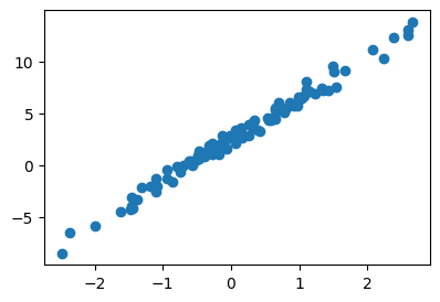
오늘 바깥의 온도는 0.5도 이다. 아이스 아메라카노를 몇잔정도 만들어 두면 좋을까?
B. 가짜자료를 만든 방법
- 방법1: \(y_i= w_0+w_1 x_i +\epsilon_i = 2.5 + 4x_i +\epsilon_i, \quad i=1,2,\dots,n\)
torch.manual_seed(43052)
x,_ = torch.randn(100).sort()
eps = torch.randn(100)*0.5
y = x * 4 + 2.5 + epsx[:5], y[:5](tensor([-2.4821, -2.3621, -1.9973, -1.6239, -1.4792]),
tensor([-8.5420, -6.5767, -5.9496, -4.4794, -4.2516]))- 방법2: \({\bf y}={\bf X}{\bf W} +\boldsymbol{\epsilon}\)
- \({\bf y}=\begin{bmatrix} y_1 \\ y_2 \\ \dots \\ y_n\end{bmatrix}, \quad {\bf X}=\begin{bmatrix} 1 & x_1 \\ 1 & x_2 \\ \dots \\ 1 & x_n\end{bmatrix}, \quad {\bf W}=\begin{bmatrix} 2.5 \\ 4 \end{bmatrix}, \quad \boldsymbol{\epsilon}= \begin{bmatrix} \epsilon_1 \\ \dots \\ \epsilon_n\end{bmatrix}\)
X = torch.stack([torch.ones(100),x],axis=1)
W = torch.tensor([[2.5],[4.0]])
y = X@W + eps.reshape(100,1)
x = X[:,[1]]X[:5,:], y[:5,:](tensor([[ 1.0000, -2.4821],
[ 1.0000, -2.3621],
[ 1.0000, -1.9973],
[ 1.0000, -1.6239],
[ 1.0000, -1.4792]]),
tensor([[-8.5420],
[-6.5767],
[-5.9496],
[-4.4794],
[-4.2516]]))- ture와 observed data를 동시에 시각화
plt.plot(x,y,'o',label=r"observed data: $(x_i,y_i)$")
#plt.plot(x,2.5+4*x,'--',label=r"true: $(x_i, 4x_i+2.5)$ // $y=4x+2.5$ ")
plt.legend()
C. 회귀분석이란?
- 클리셰: 관측한 자료 \((x_i,y_i)\) 가 있음 \(\to\) 우리는 \((x_i,y_i)\)의 관계를 파악하여 새로운 \(x\)가 왔을때 그것에 대한 예측값(predicted value) \(\hat{y}\)을 알아내는 법칙을 알고 싶음 \(\to\) 관계를 파악하기 위해서 \((x_i, y_i)\)의 산점도를 그려보니 \(x_i\)와 \(y_i\)는 선형성을 가지고 있다는 것이 파악됨 \(\to\) 오차항이 등분산성을 가지고 어쩌고 저쩌고… \(\to\) 하여튼 \((x_i,y_i)\) 를 “적당히 잘 관통하는” 어떠한 하나의 추세선을 잘 추정하면 된다.
- 회귀분석이란 산점도를 보고 적당한 추세선을 찾는 것이다. 좀 더 정확하게 말하면 \((x_1,y_1) \dots (x_n,y_n)\) 으로 \(\begin{bmatrix} \hat{w}_0 \\ \hat{w}_1 \end{bmatrix}\) 를 최대한 \(\begin{bmatrix} 2.5 \\ 4 \end{bmatrix}\)와 비슷하게 찾는 것.
given data : \(\big\{(x_i,y_i) \big\}_{i=1}^{n}\)
parameter: \({\bf W}=\begin{bmatrix} w_0 \\ w_1 \end{bmatrix}\)
estimated parameter: \({\bf \hat{W}}=\begin{bmatrix} \hat{w}_0 \\ \hat{w}_1 \end{bmatrix}\)
- 더 쉽게 말하면 아래의 그림을 보고 “적당한” 추세선을 찾는 것이다.
plt.plot(x,y,'o',label=r"observed data: $(x_i,y_i)$")
plt.legend()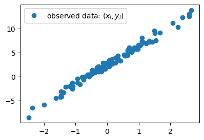
- 추세선을 그리는 행위 = \((w_0,w_1)\)을 선택하는일
4. 손실함수
# 예제1 – \((\hat{w}_0,\hat{w}_1)=(-5,10)\)을 선택하여 선을 그려보고 적당한지 판단해보자
plt.plot(x,y,'o',label=r"observed data: $(x_i,y_i)$")
What = torch.tensor([[-5.0],[10.0]])
plt.plot(x,X@What,'--',label=r"estimated line: $(x_i,\hat{y}_i)$")
plt.legend()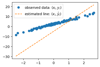
#
# 예제2 – \((\hat{w}_0,\hat{w}_1)=(2.5,3.5)\)을 선택하여 선을 그려보고 적당한지 판단해보자
plt.plot(x,y,'o',label=r"observed data: $(x_i,y_i)$")
What = torch.tensor([[2.5],[3.5]])
plt.plot(x,X@What,'--',label=r"estimated line: $(x_i,\hat{y}_i)$")
plt.legend()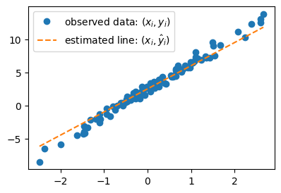
#
# 예제3 – \((\hat{w}_0,\hat{w}_1)=(2.3,3.5)\)을 선택하여 선을 그려보고 적당한지 판단해보자
plt.plot(x,y,'o',label=r"observed data: $(x_i,y_i)$")
What = torch.tensor([[2.3],[3.5]])
plt.plot(x,X@What,'--',label=r"estimated line: $(x_i,\hat{y}_i)$")
plt.legend()
plt.plot(x,y,'o',label=r"observed data: $(x_i,y_i)$")
What = torch.tensor([[2.3],[3.5]])
plt.plot(x,X@What,'--',label=r"estimated: $(x_i,\hat{y}_i)$")
plt.legend()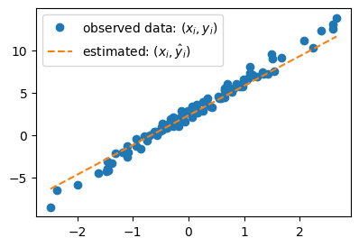
#
# 예제4 – 예제2의 추세선과 예제3의 추세선 중 뭐가 더 적당한가?
- (고민) 왠지 예제2가 더 적당하다고 답해야할 것 같은데.. 육안으로 판단하기 까다롭다..
- 적당함을 수식화 할 수 없을까?
- “적당한 정도”를 판단하기 위한 장치: loss의 개념 도입
- \(loss = \sum_{i=1}^{n}(y_i- \hat{y}_i)^2 = \sum_{i=1}^{n}\big(y_i - (\hat{w}_0+\hat{w}_1x_i)\big)^2\)
- \(loss=({\bf y}-\hat{\bf y})^\top({\bf y}-\hat{\bf y})=({\bf y}-{\bf X}\hat{\bf W})^\top({\bf y}-{\bf X}\hat{\bf W})\)
- loss의 특징
- \(y_i \approx \hat{y}_i\) 일수록 loss 값이 작음
- \(y_i \approx \hat{y}_i\) 이 되도록 \((\hat{w}_0, \hat{w}_1)\)을 잘 찍으면 loss 값이 작음
- 주황색 점선이 “적당할수록” loss 값이 작음 (그럼 우리 의도대로 된거네?)
- loss를 써먹어보자.
What = torch.tensor([[2.5],[3.5]]) # 예제2에서 찍은 What값
print(f"loss: {torch.sum((y - X@What)**2)}")

What = torch.tensor([[2.3],[3.5]]) # 예제3에서 찍은 What값
print(f"loss: {torch.sum((y - X@What)**2)}")
loss: 55.074012756347656
loss: 59.3805046081543What = torch.tensor([[2.5],[3.5]]) # 예제2에서 찍은 What값
print(f"loss: {(y - X@What).T @ (y - X@What)}")
What = torch.tensor([[2.3],[3.5]]) # 예제3에서 찍은 What값
print(f"loss: {(y - X@What).T @ (y - X@What)}")loss: tensor([[55.0740]])
loss: tensor([[59.3805]])#
5. 파이토치를 이용한 반복추정
- 추정의 전략 (손실함수도입 + 경사하강법)
- 1단계: 아무 점선이나 그어본다..
- 2단계: 1단계에서 그은 점선보다 더 좋은 점선으로 바꾼다. (=1단계에서 그은 점선보다 손실값이 작은 하나의 직선을 찾는다)
- 3단계: 1-2단계를 반복한다.
A. 1단계 – 최초의 점선
What = torch.tensor([[-5.0],[10.0]])
What
tensor([[-5.],
[10.]])yhat = X@What plt.plot(x,y,'o')
plt.plot(x,yhat.data,'--')
B. 2단계 – update
- ’적당한 정도’를 판단하기 위한 장치: loss function 도입!
\[\begin{align*} loss=& \sum_{i=1}^{n}(y_i-\hat{y}_i)^2=\sum_{i=1}^{n}(y_i-(\hat{w}_0+\hat{w}_1x_i))^2\\ =&({\bf y}-{\bf\hat{y}})^\top({\bf y}-{\bf\hat{y}})=({\bf y}-{\bf X}{\bf \hat{W}})^\top({\bf y}-{\bf X}{\bf \hat{W}}) \end{align*}\]
- loss 함수의 특징: 위 그림의 주황색 점선이 ‘적당할 수록’ loss값이 작다.
plt.plot(x,y,'o')
plt.plot(x,yhat)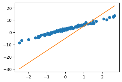
loss = torch.sum((y-yhat)**2)
losstensor(8587.6875)- 우리의 목표: 이 loss(=8587.6275)을 더 줄이자.
- 궁극적으로는 아예 모든 조합 \((\hat{w}_0,\hat{w}_1)\)에 대하여 가장 작은 loss를 찾으면 좋겠다.
- 문제의 치환: 생각해보니까 우리의 문제는 아래와 같이 수학적으로 단순화 되었다.
- 가장 적당한 주황색 선을 찾자 \(\to\) \(loss(\hat{w}_0,\hat{w}_1)\)를 최소로하는 \((\hat{w}_0,\hat{w}_1)\)의 값을 찾자.
- 수정된 목표: \(loss(\hat{w}_0,\hat{w}_1)\)를 최소로 하는 \((\hat{w}_0,\hat{w}_1)\)을 구하라.
- 단순한 수학문제가 되었다. 이것은 마치 \(f(x,y)\)를 최소화하는 \((x,y)\)를 찾으라는 것임.
- 함수의 최대값 혹은 최소값을 컴퓨터를 이용하여 찾는것을 “최적화”라고 하며 이는 산공교수님들이 가장 잘하는 분야임. (산공교수님들에게 부탁하면 잘해줌, 산공교수님들은 보통 최적화해서 어디에 쓸지보다 최적화 자체에 더 관심을 가지고 연구하심)
- 최적화를 하는 방법? 경사하강법
# 경사하강법 아이디어 (1차원)
- 임의의 점을 찍는다.
- 그 점에서 순간기울기를 구한다. (접선) <– 미분
- 순간기울기(=미분계수)의 부호를 살펴보고 부호와 반대방향으로 움직인다.
팁: 기울기의 절대값 크기와 비례하여 보폭(=움직이는 정도)을 조절한다. \(\to\) \(\alpha\)를 도입
최종수식: \(\hat{w} \leftarrow \hat{w} - \alpha \times \frac{\partial}{\partial w}loss(w)\)
#
# 경사하강법 아이디어 (2차원)
- 임의의 점을 찍는다.
- 그 점에서 순간기울기를 구한다. (접평면) <– 편미분
- 순간기울기(=미분계수)의 부호를 살펴보고 부호와 반대방향으로 각각 움직인다.
팁: 여기서도 기울기의 절대값 크기와 비례하여 보폭(=움직이는 정도)을 각각 조절한다. \(\to\) \(\alpha\)를 도입.
#
- 경사하강법 = loss를 줄이도록 \({\bf \hat{W}}\)를 개선하는 방법
- 업데이트 공식: 수정값 = 원래값 - \(\alpha\) \(\times\) 기울어진크기(=미분계수)
- 여기에서 \(\alpha\)는 전체적인 보폭의 크기를 결정한다. 즉 \(\alpha\)값이 클수록 한번의 update에 움직이는 양이 크다.
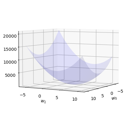
- loss는 \(\hat{\bf W} =\begin{bmatrix} \hat{w}_0 \\ \hat{w}_1 \end{bmatrix}\) 에 따라서 값이 바뀌는 함수로 해석가능하고 구체적인 형태는 아래와 같음.
- \(loss(\hat{w}_0,\hat{w}_1) =\sum_{i=1}^{n}(y_i-(\hat{w}_0+\hat{w}_1x_i))^2\)
- \(loss(\hat{\bf W})=({\bf y}-{\bf X}{\bf \hat{W}})^\top({\bf y}-{\bf X}{\bf \hat{W}})\)
따라서 구하고 싶은것은 아래와 같음
\[\hat{\bf W}^{LSE} = \underset{\bf \hat{W}}{\operatorname{argmin}} ~ loss(\hat{\bf W})\]
Warning
아래의 수식
\[\hat{\bf W}^{LSE} = \underset{\bf \hat{W}}{\operatorname{argmin}} ~ loss(\hat{\bf W})\]
은 아래와 같이 표현해도 무방합니다.
\[\hat{\bf W} = \underset{\bf W}{\operatorname{argmin}} ~ loss({\bf W})\]
마치 함수 \(f(\hat{x})=({\hat x}-1)^2\) 을 \(f(x)=(x-1)^2\) 이라고 표현할 수 있는 것 처럼요..
여기까지 01wk-2에서 수업했습니다~
여기부터는 02wk-1에서..
# 지난시간 복습
# x,X,W,y // X = [1 x], W = [w0, w1]' # 회귀분석에서는 W=β
# 회귀모형: y=X@W+ϵ = X@β+ϵ
# true: E(y)=X@W
# observed: (x,y)
# estimated W = What = [w0hat, w1hat]' <-- 아무값이나넣었음..
# estimated y = yhat = X@What = X@β̂
# loss = yhat이랑 y랑 얼마나 비슷한지 = sum((y-yhat)^2)
# (x,y) 보고 최적의 선분을 그리는것 = loss를 가장 작게 만드는 What = [w0hat, w1hat] 를 찾는것
# 전략: (1) 아무 What나 찍는다 (2) 그거보다 더 나은 What을 찾는다. (3) 1-2를 반복한다.
# 전략2가 어려운데, 이를 수행하는 방법이 경사하강법
# 경사하강법 알고리즘: 더나은What = 원래What - 0.1*미분값
What = torch.tensor([[-5.0],[10.0]])
Whattensor([[-5.],
[10.]])yhat = X@What
plt.plot(x,y,'o')
plt.plot(x,yhat,'--')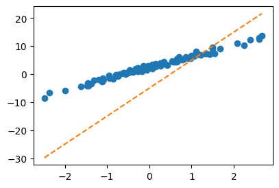
loss = torch.sum((y-yhat)**2)
losstensor(8587.6875)복습끝~
#
- 더 나은 선으로 업데이트하기 위해서는 공식 “더나은What = 원래What - 0.1*미분값” 를 적용해야하고 이를 위해서는 미분값을 계산할 수 있어야 함.
Important
경사하강법을 좀 더 엄밀하게 써보자. 경사하강법은 \(loss(\hat{\bf W})\)를 최소로 만드는 \(\hat{\bf W}\)를 컴퓨터로 구하는 방법인데, 구체적으로는 아래와 같다.
1. 임의의 점 \(\hat{\bf W}\)를 찍는다.
2. 그 점에서 순간기울기를 구한다. 즉 \(\left.\frac{\partial}{\partial {\bf W}}loss({\bf W})\right|_{{\bf W}=\hat{\bf W}}\) 를 계산한다.
3. \(\hat{\bf W}\)에서의 순간기울기의 부호를 살펴보고 부호와 반대방향으로 움직인다. 이때 기울기의 절대값 크기와 비례하여 보폭(=움직이는 정도)을 각각 조절한다. 즉 아래의 수식에 따라 업데이트 한다.
- \(\hat{\bf W} \leftarrow \hat{\bf W} - \alpha \times \left.\frac{\partial}{\partial {\bf W}}loss({\bf W})\right|_{{\bf W}=\hat{\bf W}}\)
여기에서 맨 마지막 수식을 간단하게 쓴 것이 더나은What = 원래What - 0.1*미분값 이다.
- 미분값을 계산하는 방법1
# 손실 8587.6875 를 계산하는 또 다른 방식
def l(w0,w1):
    yhat = w0 + w1*x
return torch.sum((y-yhat)**2)l(-5,10)tensor(8587.6875)h=0.001
print((l(-5+h,10) - l(-5,10))/h)
print((l(-5,10+h) - l(-5,10))/h)tensor(-1341.7968)
tensor(1190.4297)일단 이거로 업데이트해볼까?
# 더나은What = 원래What - 0.1*미분값
# [-5,10] - 0.001 * [-1341.7968,1190.4297]
sssss = What - 0.001 * torch.tensor([[-1341.7968],[1190.4297]])
ssssstensor([[-3.6582],
[ 8.8096]])plt.plot(x,y,'o')
plt.plot(x,X@What,'-') # 원래What: 주황색
plt.plot(x,X@sssss,'-') # 더나은What: 초록색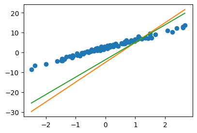
- 잘 된 것 같긴한데..
- 미분구하는게 너무 어려워..
- 다른 방법 없을까?
Important
사실 이 방법은
- \(\frac{\partial}{\partial w_0}loss(w_0,w_1) \approx \frac{loss(w_0+h,w_1)-loss(w_0,w_1)}{h}\)
- \(\frac{\partial}{\partial w_1}loss(w_0,w_1) \approx \frac{loss(w_0,w_1+h)-loss(w_0,w_1)}{h}\)
이 계산을 이용하여
- \(\frac{\partial}{\partial {\bf W}}loss({\bf W}):= \begin{bmatrix} \frac{\partial}{\partial w_0} \\ \frac{\partial}{\partial w_1}\end{bmatrix}loss({\bf W}) = \begin{bmatrix} \frac{\partial}{\partial w_0}loss({\bf W}) \\ \frac{\partial}{\partial w_1}loss({\bf W})\end{bmatrix} = \begin{bmatrix} \frac{\partial}{\partial w_0}loss(w_0,w_1) \\ \frac{\partial}{\partial w_1}loss(w_0,w_1)\end{bmatrix}\)
를 계산한 것이라 볼 수 있죠
- 미분값을 계산하는 방법2
## 약간의 지식이 필요함.
# loss = (y-XWhat)'(y-XWhat)
# = (y'-What'X')(y-XWhat)
# = y'y-y'XWhat -What'X'y + What'X'XWhat
# loss를 What으로 미분
# loss' = -X'y - X'y + 2X'XWhat-2*X.T@y + 2*X.T@X@Whattensor([[-1342.2524],
[ 1188.9302]])
Important
이 방법은 \(loss({\bf W})\)의 미분을 구할수 있어야 사용가능합니다. 즉
\[\frac{\partial}{\partial {\bf W}}loss({\bf W})= -2{\bf X}^\top {\bf y} + 2{\bf X}^\top {\bf X}{\bf W}\]
를 계산할 수 있어야 합니다.
- 미분값을 계산하는 방법3 – 이 패턴을 외우세여
What = torch.tensor([[-5.0],[10.0]],requires_grad=True)
What
tensor([[-5.],
[10.]], requires_grad=True)yhat = X@What
loss = torch.sum((y-yhat)**2)
losstensor(8587.6875, grad_fn=<SumBackward0>)loss.backward() # loss를 미분하라.. 꼬리표가 있게 한 What으로.. What.gradtensor([[-1342.2524],
[ 1188.9305]])- 위의 코드를 다시 복습해보자.
– loss.backward()실행전 –
What = torch.tensor([[-5.0],[10.0]],requires_grad=True)
yhat = X@What
loss = torch.sum((y-yhat)**2)What.data, What.grad(tensor([[-5.],
[10.]]),
None)– loss.backward()실행후 –
loss.backward()What.data, What.grad(tensor([[-5.],
[10.]]),
tensor([[-1342.2524],
[ 1188.9305]]))# 1회 업데이트 과정을 차근차근 시각화하며 정리해보자.
alpha = 0.001
print(f"{What.data} -- 수정전")
print(f"{-alpha*What.grad} -- 수정하는폭")
print(f"{What.data-alpha*What.grad} -- 수정후")
print(f"{torch.tensor([[2.5],[4]])} -- 참값(이건 비밀~~)")tensor([[-5.],
[10.]]) -- 수정전
tensor([[ 1.3423],
[-1.1889]]) -- 수정하는폭
tensor([[-3.6577],
[ 8.8111]]) -- 수정후
tensor([[2.5000],
[4.0000]]) -- 참값(이건 비밀~~)Wbefore = What.data
Wafter = What.data - alpha * What.grad
Wbefore, Wafter(tensor([[-5.],
[10.]]),
tensor([[-3.6577],
[ 8.8111]]))plt.plot(x,y,'o',label=r'observed data')
plt.plot(x,X@Wbefore,'--', label=r"$\hat{\bf y}_{before}={\bf X}@\hat{\bf W}_{before}$")
plt.plot(x,X@Wafter,'--', label=r"$\hat{\bf y}_{after}={\bf X}@\hat{\bf W}_{after}$")
plt.legend()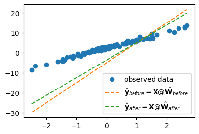
#
C. 3단계 – iteration (=learn = estimate \(\bf{\hat W}\))
- 이제 1단계와 2단계를 반복만하면된다. 그래서 아래와 같은 코드를 작성하면 될 것 같은데…
What = torch.tensor([[-5.0],[10.0]],requires_grad=True) # 최초의 직선을 만드는 값
for epoc in range(30):
yhat = X@What
loss = torch.sum((y-yhat)**2)
loss.backward()
What.data = What.data - 0.001 * What.grad돌려보면 잘 안된다.
- 아래와 같이 해야한다.
What = torch.tensor([[-5.0],[10.0]],requires_grad=True) # 최초의 직선을 만드는 값
for epoc in range(30):
    yhat = X@What
    loss = torch.sum((y-yhat)**2)
    loss.backward()
    What.data = What.data - 0.001 * What.grad
What.grad = None plt.plot(x,y,'o',label=r"observed: $(x_i,y_i)$")
plt.plot(x,X@What.data,'--o', label=r"estimated: $(x_i,\hat{y}_i)$ -- after 30 iterations (=epochs)", alpha=0.4 )
plt.legend()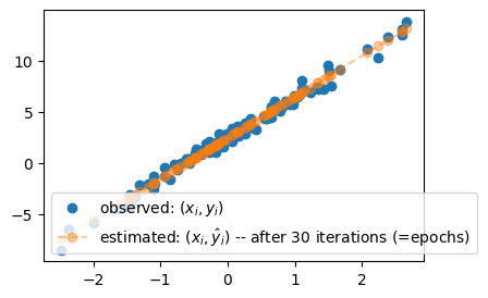
- 왜? loss.backward() 는 아래의 역할을 하는것 처럼 이해되었지만
What.grad\(\leftarrow\)What에서미분값
실제로는 아래의 역할을 수행하기 때문이다. (컴퓨터공학적인 이유로..)
What.grad\(\leftarrow\)What.grad+What에서미분값
Note
What.grad \(\leftarrow\) What.grad + What에서미분값 임을 확인하기 위해서.. 약간의 테스트를 했습니다.
먼저
What = torch.tensor([[-5.0],[10.0]],requires_grad=True) # 최초의 직선을 만드는 값
print(What.data)
print(What.grad)
를 확인한뒤 아래를 반복실행해봤을때
yhat = X@What
loss = torch.sum((y-yhat)**2)
loss.backward() #
print(What.data)
print(What.grad)What.data와 What.grad 값이 계속 일정하게 나온다면
What.grad\(\leftarrow\)What에서미분값
이와 같은 계산이 진행되는 것이겠고, What.grad의 값이 자꾸 커진다면
What.grad\(\leftarrow\)What.grad+What에서미분값
이와 같은 계산이 진행되는 것이겠죠?