13wk-1: 순환신경망 (4) – LSTM 계산과정 재현, LSTM은 왜 강한가?

1. 강의영상

2. Import

import torch
import pandas as pd
import matplotlib.pyplot as plt

soft = torch.nn.Softmax(dim=1)
sig = torch.nn.Sigmoid()
tanh = torch.nn.Tanh()

3. Data – abcabC

txt = list('abcabC')*50
txt[:10]

['a', 'b', 'c', 'a', 'b', 'C', 'a', 'b', 'c', 'a']

df_train = pd.DataFrame({'x':txt[:-1], 'y':txt[1:]})
df_train[:5]

	x	y
0	a	b
1	b	c
2	c	a
3	a	b
4	b	C

x = torch.tensor(df_train.x.map({'a':0,'b':1,'c':2,'C':3}))
y = torch.tensor(df_train.y.map({'a':0,'b':1,'c':2,'C':3}))
X = torch.nn.functional.one_hot(x).float()
y = torch.nn.functional.one_hot(y).float()

4. LSTM 계산과정 재현

A. torch.nn.LSTMCell

torch.manual_seed(43052)
lstmcell = torch.nn.LSTMCell(4,2) # 숙성담당
cook = torch.nn.Linear(2,4)
loss_fn = torch.nn.CrossEntropyLoss()
optimizr = torch.optim.Adam(list(lstmcell.parameters())+list(cook.parameters()),lr=0.1) 
#---#
L = len(X)
for epoc in range(1):
    # 1~2 
    loss = 0 
    ht = torch.zeros(2)
    ct = torch.zeros(2)
    for t in range(L):
        Xt,yt = X[t],y[t]
        ht,ct = lstmcell(Xt,(ht,ct))
        netout_t = cook(ht)
        loss = loss + loss_fn(netout_t,yt) 
    loss = loss/L
    # 3
    loss.backward()
    # 4 
    optimizr.step()
    optimizr.zero_grad()

ht,ct

(tensor([0.0533, 0.2075], grad_fn=<SqueezeBackward1>),
 tensor([0.1218, 0.5590], grad_fn=<SqueezeBackward1>))

B. 직접구현

t=0 \(\to\) t=1

- lstmcell을 이용하여 \(t=0 \to t=1\)을 구현해보자. (결과비교용)

torch.manual_seed(43052)
lstmcell = torch.nn.LSTMCell(4,2) # 숙성담당
cook = torch.nn.Linear(2,4)
loss_fn = torch.nn.CrossEntropyLoss()
optimizr = torch.optim.Adam(list(lstmcell.parameters())+list(cook.parameters()),lr=0.1) 
#---#
L = len(X)
for epoc in range(1):
    # 1~2 
    loss = 0 
    ht = torch.zeros(2)
    ct = torch.zeros(2)
    for t in range(1):
        Xt,yt = X[t],y[t]
        ht,ct = lstmcell(Xt,(ht,ct))
        netout_t = cook(ht)
        loss = loss + loss_fn(netout_t,yt) 
    loss = loss/L
    # 3
    loss.backward()
    # 4 
    optimizr.step()
    optimizr.zero_grad()

ht,ct

(tensor([0.1067, 0.1069], grad_fn=<SqueezeBackward1>),
 tensor([0.1734, 0.2688], grad_fn=<SqueezeBackward1>))

• 이런결과를 어떻게 만드는걸까?
• https://pytorch.org/docs/stable/generated/torch.nn.LSTM.html

- 직접계산 (\({\boldsymbol i}_t, {\boldsymbol f}_t, {\boldsymbol g}_t, {\boldsymbol o}_t\))

torch.manual_seed(43052)
lstmcell = torch.nn.LSTMCell(4,2) # 숙성담당

Wih = lstmcell.weight_ih.T
Wih02 = Wih[:,0:2]
Wih24 = Wih[:,2:4]
Wih46 = Wih[:,4:6]
Wih68 = Wih[:,6:8]
#--#
Whh = lstmcell.weight_hh.T
Whh02 = Whh[:,0:2]
Whh24 = Whh[:,2:4]
Whh46 = Whh[:,4:6]
Whh68 = Whh[:,6:8]
#--#
bih02 = lstmcell.bias_ih[0:2]
bih24 = lstmcell.bias_ih[2:4]
bih46 = lstmcell.bias_ih[4:6]
bih68 = lstmcell.bias_ih[6:8]
#--#
bhh02 = lstmcell.bias_hh[0:2]
bhh24 = lstmcell.bias_hh[2:4]
bhh46 = lstmcell.bias_hh[4:6]
bhh68 = lstmcell.bias_hh[6:8]

ht = torch.zeros(2)
ct = torch.zeros(2)
#--#
it = sig(Xt@Wih02 + bih02 + ht@Whh02 + bhh02)
ft = sig(Xt@Wih24 + bih24 + ht@Whh24 + bhh24)
gt = tanh(Xt@Wih46 + bih46 + ht@Whh46 + bhh46)
ot = sig(Xt@Wih68 + bih68 + ht@Whh68 + bhh68)

it,ft,gt,ot

(tensor([0.3081, 0.5949], grad_fn=<SigmoidBackward0>),
 tensor([0.5065, 0.4264], grad_fn=<SigmoidBackward0>),
 tensor([0.5629, 0.4518], grad_fn=<TanhBackward0>),
 tensor([0.6216, 0.4072], grad_fn=<SigmoidBackward0>))

그런데 아래와 같이 계산할수도 있음.

ifgo = Xt @ lstmcell.weight_ih.T +  lstmcell.bias_ih +\
ht @ lstmcell.weight_hh.T +  lstmcell.bias_hh

print(f"it = {sig(ifgo[0:2])}")
print(f"ft = {sig(ifgo[2:4])}")
print(f"gt = {tanh(ifgo[4:6])}")
print(f"ot = {sig(ifgo[6:8])}")

it = tensor([0.3081, 0.5949], grad_fn=<SigmoidBackward0>)
ft = tensor([0.5065, 0.4264], grad_fn=<SigmoidBackward0>)
gt = tensor([0.5629, 0.4518], grad_fn=<TanhBackward0>)
ot = tensor([0.6216, 0.4072], grad_fn=<SigmoidBackward0>)

- 직접계산 (\({\boldsymbol c}_t, {\boldsymbol h}_t\))

ct = it*gt + ft*ct 
ht = ot*tanh(ct)

ht,ct

(tensor([0.1067, 0.1069], grad_fn=<MulBackward0>),
 tensor([0.1734, 0.2688], grad_fn=<AddBackward0>))

# t=0 \(\to\) t=L

- lstmcell을 이용하여 구현해보자. (결과비교용)

torch.manual_seed(43052)
lstmcell = torch.nn.LSTMCell(4,2) # 숙성담당
cook = torch.nn.Linear(2,4)
loss_fn = torch.nn.CrossEntropyLoss()
optimizr = torch.optim.Adam(list(lstmcell.parameters())+list(cook.parameters()),lr=0.1) 
#---#
L = len(X)
for epoc in range(1):
    # 1~2 
    loss = 0 
    ht = torch.zeros(2)
    ct = torch.zeros(2)
    for t in range(L):
        Xt,yt = X[t],y[t]
        ht,ct = lstmcell(Xt,(ht,ct))
        netout_t = cook(ht)
        loss = loss + loss_fn(netout_t,yt) 
    loss = loss/L
    # 3
    loss.backward()
    # 4 
    optimizr.step()
    optimizr.zero_grad()

ht,ct

(tensor([0.0533, 0.2075], grad_fn=<SqueezeBackward1>),
 tensor([0.1218, 0.5590], grad_fn=<SqueezeBackward1>))

- 직접구현

torch.manual_seed(43052)
lstmcell = torch.nn.LSTMCell(4,2) # 숙성담당
cook = torch.nn.Linear(2,4)
loss_fn = torch.nn.CrossEntropyLoss()
optimizr = torch.optim.Adam(list(lstmcell.parameters())+list(cook.parameters()),lr=0.1) 
#---#
L = len(X)
for epoc in range(1):
    # 1~2 
    loss = 0 
    ht = torch.zeros(2)
    ct = torch.zeros(2)
    for t in range(L):
        Xt,yt = X[t],y[t]
        ifgo = Xt @ lstmcell.weight_ih.T +  lstmcell.bias_ih +\
                ht @ lstmcell.weight_hh.T +  lstmcell.bias_hh
        it,ft,gt,ot = sig(ifgo[0:2]),sig(ifgo[2:4]),tanh(ifgo[4:6]),sig(ifgo[6:8])
        ct = it*gt + ft*ct
        ht = ot*tanh(ct)
        netout_t = cook(ht)
        loss = loss + loss_fn(netout_t,yt) 
    loss = loss/L
    # 3
    loss.backward()
    # 4 
    optimizr.step()
    optimizr.zero_grad()

ht,ct

(tensor([0.0533, 0.2075], grad_fn=<MulBackward0>),
 tensor([0.1218, 0.5590], grad_fn=<AddBackward0>))

C. torch.nn.LSTM

torch.manual_seed(43052)
lstmcell = torch.nn.LSTMCell(4,2) # 숙성담당
cook = torch.nn.Linear(2,4)
lstm = torch.nn.LSTM(4,2) # <-- 이거로 학습
lstm.weight_ih_l0.data = lstmcell.weight_ih.data
lstm.weight_hh_l0.data = lstmcell.weight_hh.data
lstm.bias_ih_l0.data = lstmcell.bias_ih.data
lstm.bias_hh_l0.data = lstmcell.bias_hh.data
loss_fn = torch.nn.CrossEntropyLoss()
optimizr = torch.optim.Adam(list(lstm.parameters())+list(cook.parameters()),lr=0.1) 
#---#
L = len(X)
Water = torch.zeros(1,2)
for epoc in range(1):
    # 1 
    h,(hL,cL) = lstm(X,(Water,Water))
    netout = cook(h)
    # 2 
    loss = loss_fn(netout,y)
    # 3
    loss.backward()
    # 4 
    optimizr.step()
    optimizr.zero_grad()

hL,cL

(tensor([[0.0533, 0.2075]], grad_fn=<SqueezeBackward1>),
 tensor([[0.1218, 0.5590]], grad_fn=<SqueezeBackward1>))

5. LSTM은 왜 강한가?

A. 적합 및 시각화

- 적합

torch.manual_seed(43052)
lstm = torch.nn.LSTM(4,2)
cook = torch.nn.Linear(2,4)
loss_fn = torch.nn.CrossEntropyLoss() 
optimizr = torch.optim.Adam(list(lstm.parameters())+ list(cook.parameters()),lr=0.1)
#--#
Water = torch.zeros(1,2) 
for epoc in range(200): 
    ## step1 
    h, (hL,cL) = lstm(X,(Water,Water))
    netout = cook(h)
    ## step2
    loss = loss_fn(netout,y) 
    ## step3
    loss.backward()
    ## step4 
    optimizr.step()
    optimizr.zero_grad() 

- 시각화

L = len(X)
i = input_gate = torch.zeros(L,2)
f = forget_gate = torch.zeros(L,2)
g = gihhen_state = torch.zeros(L,2)
o = output_gate = torch.zeros(L,2)
c = cell_state = torch.zeros(L,2)
h = hidden_state = torch.zeros(L,2) 
#--#
water = torch.zeros(2)
ifgo = X[0] @ lstm.weight_ih_l0.T + lstm.bias_ih_l0 +\
        water @ lstm.weight_hh_l0.T + lstm.bias_hh_l0 
# 위에서 water는 h0에 대응
i[0] = sig(ifgo[0:2])
f[0] = sig(ifgo[2:4])
g[0] = tanh(ifgo[4:6])
o[0] = sig(ifgo[6:8])
c[0] = f[0] * water + i[0] * g[0] # water는 c0에 대응 
h[0] = o[0] * tanh(c[0])
#--#
for t in range(1,L): 
    ## 1: calculate ifgo 
    ifgo = X[t] @ lstm.weight_ih_l0.T + lstm.bias_ih_l0 +\
            h[t-1] @ lstm.weight_hh_l0.T +  lstm.bias_hh_l0 
    ## 2: decompose ifgo 
    i[t] = sig(ifgo[0:2])
    f[t] = sig(ifgo[2:4])
    g[t] = tanh(ifgo[4:6])
    o[t] = sig(ifgo[6:8])
    ## 3: calculate ht,ct 
    c[t] = f[t] * c[t-1] + i[t] * g[t]
    h[t] = o[t] * tanh(c[t])

mat = torch.concat([g,h,soft(netout)],axis=1)[:8].data
plt.matshow(mat,cmap='bwr',vmin=-1,vmax=1);
plt.axvline(x=3.5,color="lime")
plt.xticks(
    ticks=range(mat.shape[-1]),
    labels=[r"$g_0$",r"$g_1$",r"$h_0$",r"$h_1$",
            r"$P_a$",r"$P_b$",r"$P_c$",r"$P_C$"]
)
plt.colorbar()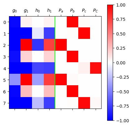

B. 시각화1: \(({\boldsymbol g}_t, {\boldsymbol c}_{t-1}) \to {\boldsymbol c}_{t}\)

mat1 = torch.concat([g[1:9],i[1:9],g[1:9]*i[1:9]],axis=1).data
mat2 = torch.concat([c[:8],f[1:9],c[:8]*f[1:9]],axis=1).data
mat3 = torch.concat([g[1:9]*i[1:9],c[:8]*f[1:9],c[1:9]],axis=1).data

c[:8].min(),c[:8].max() 

(tensor(-1.0900, grad_fn=<MinBackward1>),
 tensor(0.9979, grad_fn=<MaxBackward1>))

• \({\boldsymbol c}_t\)의 경우 원래 출력값이 -1, 1 사이라는 보장은 없으나, 이 예제의 경우에는 거의 -1, 1 사이임.
• matshow로 시각화할때 vmin=-1, vmax=1로 설정해도 \({\boldsymbol c}_t\)를 표현함에 부족함이 없을듯

fig,ax = plt.subplots(1,3,figsize=(10,10))
ax[0].matshow(mat1,cmap='bwr',vmin=-1,vmax=1);
ax[0].axvline(x=1.5,linestyle="dashed",color="lime")
ax[0].axvline(x=3.5,linestyle="dashed",color="lime")
ax[0].set_xticks(ticks= [0.5,2.5,4.5],labels=[r'${\bf g}_t$',r'${\bf i}_t$',r'${\bf g}_t \odot {\bf i}_t$']);
ax[1].matshow(mat2,cmap='bwr',vmin=-1,vmax=1);
ax[1].axvline(x=1.5,linestyle="dashed",color="lime")
ax[1].axvline(x=3.5,linestyle="dashed",color="lime")
ax[1].set_xticks(ticks= [0.5,2.5,4.5],labels=[r'${\bf c}_{t-1}$',r'${\bf f}_t$',r'${\bf c}_{t-1} \odot {\bf f}_t$']);
ax[2].matshow(mat3,cmap='bwr',vmin=-1,vmax=1);
ax[2].axvline(x=1.5,linestyle="dashed",color="lime")
ax[2].axvline(x=3.5,linestyle="dashed",color="lime")
ax[2].set_xticks(ticks= [0.5,2.5,4.5],labels=[r'${\bf g}_t \odot {\bf i}_t$',r'${\bf c}_{t-1} \odot {\bf f}_t$',r'${\bf c}_t$']);
fig.tight_layout()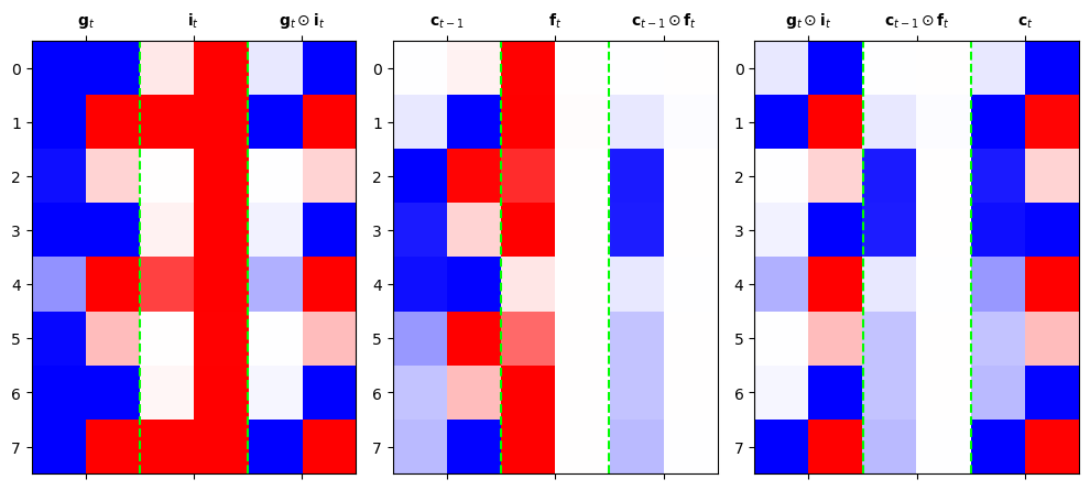

- \({\boldsymbol g}_t\) 특징: 보통 -1,1 중 하나의 값을 가지도록 학습되어 있다. (마치 RNN의 hidden node처럼!)

• \(\boldsymbol{g}_t = \tanh({\boldsymbol x}_t {\bf W}_{ig} + {\boldsymbol h}_{t-1} {\bf W}_{hg}+ {\boldsymbol b}_{ig}+{\boldsymbol b}_{hg})\)

- \({\boldsymbol c}_t\) 특징: \({\boldsymbol g}_t\)와 매우 비슷하지만 약간 다른값을 가진다. 그래서 \({\boldsymbol g}_t\)와는 달리 -1,1 이외의 값도 종종 등장.

• \({\boldsymbol c}_t\)의 값은 이론상 제한이 없음. (꼭 -1,1 사이에 있지 않음)

C. 시각화2: \({\boldsymbol g}_t \to {\boldsymbol h}_{t}\)

mat = torch.concat([g[:8],tanh(c[:8]),o[:8],h[:8]],axis=1).data

plt.matshow(mat.data,cmap='bwr',vmin=-1,vmax=1)
plt.xticks([0.5,2.5,4.5,6.5],[r'${\bf g}_t$',r'$tanh({\bf c}_t)$',r'${\bf o}_t$',r'${\bf h}_t$']);
plt.axvline(x=1.5,color="lime",linewidth=3)
plt.axvline(x=3.5,linestyle="dashed",color="lime")
plt.axvline(x=5.5,linestyle="dashed",color="lime")
plt.axvline(x=7.5,color="lime",linewidth=3)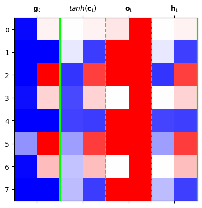

- \({\boldsymbol h}_t\) 특징: (1) \({\boldsymbol c}_t\)에서 원하는 것만 선택적으로 특징으로 삼은 느낌. (2) \(c_t\)보다 훨씬 값을 다양하게 가진다. (\(\odot\) 의 효과 )

D. LSTM의 알고리즘 리뷰 I (수식위주)

(step1) calculate \({\tt ifgo}\)

\({\tt ifgo} = {\boldsymbol x}_t \big[{\bf W}_{ii} | {\bf W}_{if}| {\bf W}_{ig} |{\bf W}_{io}\big] + {\boldsymbol h}_{t-1} \big[ {\bf W}_{hi}|{\bf W}_{hf} |{\bf W}_{hg} | {\bf W}_{ho} \big] + bias\)

\(=\big[{\boldsymbol x}_t{\bf W}_{ii} + {\boldsymbol h}_{t-1}{\bf W}_{hi} ~\big|~ {\boldsymbol x}_t{\bf W}_{if}+ {\boldsymbol h}_{t-1}{\bf W}_{hf}~ \big|~ {\boldsymbol x}_t{\bf W}_{ig} + {\boldsymbol h}_{t-1}{\bf W}_{hg} ~\big|~ {\boldsymbol x}_t{\bf W}_{io} + {\boldsymbol h}_{t-1}{\bf W}_{ho} \big] + bias\)

참고: 위의 수식은 아래코드에 해당하는 부분

ifgo = Xt @ lstm_cell.weight_ih.T +\
       ht @ lstm_cell.weight_hh.T +\
       lstm_cell.bias_ih + lstm_cell.bias_hh

(step2) decompose \({\tt ifgo}\) and get \({\boldsymbol i}_t\), \({\boldsymbol f}_t\), \({\boldsymbol g}_t\), \({\boldsymbol o}_t\)

\({\boldsymbol i}_t = \sigma({\boldsymbol x}_t {\bf W}_{ii} + {\boldsymbol h}_{t-1} {\bf W}_{hi} +bias )\)

\({\boldsymbol f}_t = \sigma({\boldsymbol x}_t {\bf W}_{if} + {\boldsymbol h}_{t-1} {\bf W}_{hf} +bias )\)

\({\boldsymbol g}_t = \tanh({\boldsymbol x}_t {\bf W}_{ig} + {\boldsymbol h}_{t-1} {\bf W}_{hg} +bias )\)

\({\boldsymbol o}_t = \sigma({\boldsymbol x}_t {\bf W}_{io} + {\boldsymbol h}_{t-1} {\bf W}_{ho} +bias )\)

(step3) calculate \({\boldsymbol c}_t\) and \({\boldsymbol h}_t\)

\({\boldsymbol c}_t = {\boldsymbol i}_t \odot {\boldsymbol g}_t+ {\boldsymbol f}_t \odot {\boldsymbol c}_{t-1}\)

\({\boldsymbol h}_t = {\boldsymbol o}_t \odot \tanh({\boldsymbol c}_t)\)

E. LSTM의 알고리즘 리뷰 II (느낌위주)

• 이해 및 암기를 돕기위해서 비유적으로 설명한 챕터입니다..

- 느낌: RNN이 콩물에서 간장을 한번에 숙성시키는 방법이라면 LSTM은 콩물에서 간장을 단계를 나누어 숙성하는 느낌이다.

• RNN: \({\boldsymbol x}_t \overset{{\boldsymbol h}_{t-1}}{\longrightarrow} {\boldsymbol h}_t\)
• LSTM: \({\boldsymbol x}_t \overset{{\boldsymbol h}_{t-1}}{\longrightarrow} {\boldsymbol g}_t \overset{{\boldsymbol c}_{t-1}}{\longrightarrow} \Big({\boldsymbol c}_t \to {\boldsymbol h}_t \Big)\)

- \({\boldsymbol g}_t\)에 대하여

• 과거와 현재의 결합 (선형변환): \({\boldsymbol x}_t\)와 \({\boldsymbol h}_{t-1}\)를 \({\bf W}_{ig}, {\bf W}_{hg}\)를 이용해 선형결합
• 숙성(비선형변환): \(\tanh\)
• 느낌: RNN에서 간장을 만들던 그 수식에서 \(h_t\)를 \(g_t\)로 바꾼것 그래서 RNN의 간장과 비슷하다고 생각하면 된다.
• 노트: RNN의 간장은 한계를 가지고 있는데 그 한계를 극복하기 위해 만든 것이 \({\boldsymbol c}_t\)

- \({\boldsymbol c}_t\)에 대하여

• 과거와 현재의 결합 (선형변환): \({\boldsymbol g}_{t}\)와 \({\boldsymbol c}_{t-1}\)를 요소별로 선택하고 더하는 과정
• 숙성 (비선형변환): 없음.
• 느낌: 과거와 현재의 정보중 유리한것만 기억하여 선택적으로 결합함. 이때 결합방식에 대한 노하우는 \({\tt input-gate}\), \({\tt forget-gate}\) 에 있으며 그러한 결합의 결과가 \({\boldsymbol c}_t\)에 있음. 이 \({\boldsymbol c}_t\)에 대한 정보는 그대로 “냉동보관(?)”되어 다음세대로 내려옴.
• 비고: \({\boldsymbol c}_t\)는 사실상 LSTM 알고리즘의 꽃이라 할 수 있음. LSTM은 long short term memory의 약자임. 기존의 RNN은 장기기억을 활용함에 약점이 있는데 LSTM은 단기기억/장기기억 모두 잘 활용함. LSTM이 장기기억을 잘 활용하는 비법은 바로 \({\boldsymbol c}_t\)에 있다.

- \({\boldsymbol h}_t\)에 대하여

• 과거와 현재의 결합 (선형변환): 없음
• 숙성 (비선형변환): \(\tanh({\boldsymbol c}_t)\)를 요소별로 선택하여 숙성

RNN은 기억할 과거정보가 \({\boldsymbol h}_{t-1}\) 하나이지만 LSTM은 \({\boldsymbol c}_{t-1}\), \({\boldsymbol h}_{t-1}\) 2개이다.

F. LSTM이 강한이유

- 답변1: LSTM이 장기기억에 유리함. 그 이유는 input, forget, output gate 들이 장기기억을 위한 역할을 하기 때문.

• 비판: 아키텍처에 대한 이론적 근거는 없음. 장기기억을 위하여 꼭 LSTM같은 구조일 필요는 없음. (게이트는 꼭3개이어야 하는지?)

- 답변2: 저는 사실 아까 살펴본 아래의 이유로 이해하고 있습니다.

• 실험적으로 살펴보니 LSTM이 RNN보다 장기기억에 유리했음.
• 그 이유: RNN은 \({\boldsymbol h}_t\)의 값이 -1 혹은 1로 결정되는 경우가 많았음. 그러나 경우에 따라서는 \({\boldsymbol h}_t\)이 -1~1의 값을 가지는 것이 문맥적 뉘앙스를 포착하기에는 유리한데 LSTM이 이러한 방식으로 학습되는 경우가 많았음.
• 왜 LSTM의 \({\boldsymbol h}_t\)은 -1,1 이외의 값을 쉽게 가질 수 있는가? \(\odot\) 때문에.. 즉 게이트때문에..

6. Ref

- 참고자료들

• https://colah.github.io/posts/2015-08-Understanding-LSTMs/
• https://pytorch.org/docs/stable/generated/torch.nn.LSTM.html
• https://arxiv.org/abs/1402.1128