06wk-1: 합성곱 신경망 (2) – MNIST, Fashion MNIST, ImageNet, CIFAR10

1. 강의영상

2. Imports

import torch
import torchvision
import matplotlib.pyplot as plt
import pandas as pd
import numpy as np
import fastai.vision.all 

3. torch.eigensum

A. transpose

tsr = torch.arange(12).reshape(4,3)
tsr

tensor([[ 0,  1,  2],
        [ 3,  4,  5],
        [ 6,  7,  8],
        [ 9, 10, 11]])

tsr.t()

tensor([[ 0,  3,  6,  9],
        [ 1,  4,  7, 10],
        [ 2,  5,  8, 11]])

torch.einsum('ij->ji',tsr)

tensor([[ 0,  3,  6,  9],
        [ 1,  4,  7, 10],
        [ 2,  5,  8, 11]])

B. 행렬곱

tsr1 = torch.arange(12).reshape(4,3).float()
tsr2 = torch.arange(15).reshape(3,5).float()

tsr1.shape

torch.Size([4, 3])

tsr2.shape

torch.Size([3, 5])

tsr1 @ tsr2

tensor([[ 25.,  28.,  31.,  34.,  37.],
        [ 70.,  82.,  94., 106., 118.],
        [115., 136., 157., 178., 199.],
        [160., 190., 220., 250., 280.]])

torch.einsum('ij,jk -> ik',tsr1,tsr2) 

tensor([[ 25.,  28.,  31.,  34.,  37.],
        [ 70.,  82.,  94., 106., 118.],
        [115., 136., 157., 178., 199.],
        [160., 190., 220., 250., 280.]])

C. 이미지변환

r = torch.zeros(16).reshape(4,4) + 1.0
g = torch.zeros(16).reshape(4,4)
b = torch.zeros(16).reshape(4,4)
img_plt = torch.stack([r,g,b],axis=-1) # matplotlib 를 쓰기 위해서는 이미지가 이렇게 저장되어있어야한다. 
img_torch = torch.stack([r,g,b],axis=0).reshape(1,3,4,4) # torch를 쓰기 위해서는 이미지가 이렇게 저장되어있어야한다. 

img_plt.shape, img_torch.shape

(torch.Size([4, 4, 3]), torch.Size([1, 3, 4, 4]))

plt.imshow(img_plt)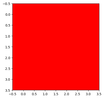

만약에 img_torch를 matplotlib 으로 보고싶다면?

# 잘못된코드
plt.imshow(img_torch.reshape(4,4,3))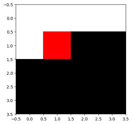

# 올바른코드
plt.imshow(torch.einsum('ocij -> ijc',img_torch))

4. MNIST – 직접설계

path = fastai.data.external.untar_data(fastai.data.external.URLs.MNIST)
X0 = torch.stack([torchvision.io.read_image(str(fname)) for fname in (path/'training/0').ls()])
X1 = torch.stack([torchvision.io.read_image(str(fname)) for fname in (path/'training/1').ls()])
X2 = torch.stack([torchvision.io.read_image(str(fname)) for fname in (path/'training/2').ls()])
X = torch.concat([X0,X1,X2])/255
y = torch.nn.functional.one_hot(torch.tensor([0]*len(X0) + [1]*len(X1) + [2]*len(X2))).float()
X0 = torch.stack([torchvision.io.read_image(str(fname)) for fname in (path/'testing/0').ls()])
X1 = torch.stack([torchvision.io.read_image(str(fname)) for fname in (path/'testing/1').ls()])
X2 = torch.stack([torchvision.io.read_image(str(fname)) for fname in (path/'testing/2').ls()])
XX = torch.concat([X0,X1,X2])/255
yy = torch.nn.functional.one_hot(torch.tensor([0]*len(X0) + [1]*len(X1) + [2]*len(X2))).float()

print(X.shape,'\t',X.dtype)
print(y.shape,'\t\t\t',y.dtype)
print(XX.shape,'\t',XX.dtype)
print(yy.shape,'\t\t\t',yy.dtype)

torch.Size([18623, 1, 28, 28])   torch.float32
torch.Size([18623, 3])           torch.float32
torch.Size([3147, 1, 28, 28])    torch.float32
torch.Size([3147, 3])            torch.float32

plt.imshow(torch.einsum('cij -> ijc',X[0]),cmap="gray")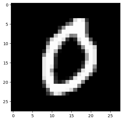

A. y: (n,3)-float

# Step1: 데이터정리 (dls생성)
ds = torch.utils.data.TensorDataset(X,y)
dl = torch.utils.data.DataLoader(ds,batch_size=128) 
# Step2: 적합에 필요한 오브젝트 생성
net1 = torch.nn.Sequential(
    torch.nn.Conv2d(1,16,(5,5)),
    torch.nn.ReLU(),
    torch.nn.MaxPool2d((2,2)),
    torch.nn.Flatten()
)
net2 = torch.nn.Sequential(
    torch.nn.Linear(2304,3),
)
net = torch.nn.Sequential(
    net1, # 2d-part
    net2, # 1d-part 
)
loss_fn = torch.nn.CrossEntropyLoss()
optimizr = torch.optim.Adam(net.parameters())
# Step3: 적합 
net.to("cuda:0")
for epoc in range(10):
    for xi,yi in dl:
        ## 1
        ## 2
        loss = loss_fn(net(xi.to("cuda:0")),yi.to("cuda:0"))
        ## 3 
        loss.backward()
        ## 4 
        optimizr.step()
        optimizr.zero_grad()
net.to("cpu")
# Step4: 예측 및 평가 
print(f'train: {(net(X).data.argmax(axis=1) == y.argmax(axis=1)).float().mean():.4f}')
print(f'val: {(net(XX).data.argmax(axis=1) == yy.argmax(axis=1)).float().mean():.4f}')

train: 0.9851
val: 0.9898

B. y: (n,)-int

y = y.argmax(axis=-1)
yy = yy.argmax(axis=-1)
y,yy

(tensor([0, 0, 0,  ..., 2, 2, 2]), tensor([0, 0, 0,  ..., 2, 2, 2]))

print(X.shape,'\t',X.dtype)
print(y.shape,'\t\t',y.dtype)
print(XX.shape,'\t',XX.dtype)
print(yy.shape,'\t\t',yy.dtype)

torch.Size([18623, 1, 28, 28])   torch.float32
torch.Size([18623])          torch.int64
torch.Size([3147, 1, 28, 28])    torch.float32
torch.Size([3147])       torch.int64

# Step1: 데이터정리 (dls생성)
ds = torch.utils.data.TensorDataset(X,y)
dl = torch.utils.data.DataLoader(ds,batch_size=128) 
# Step2: 적합에 필요한 오브젝트 생성
net1 = torch.nn.Sequential(
    torch.nn.Conv2d(1,16,(5,5)),
    torch.nn.ReLU(),
    torch.nn.MaxPool2d((2,2)),
    torch.nn.Flatten()
)
net2 = torch.nn.Sequential(
    torch.nn.Linear(2304,3),
)
net = torch.nn.Sequential(
    net1, # 2d-part
    net2, # 1d-part 
)
loss_fn = torch.nn.CrossEntropyLoss()
optimizr = torch.optim.Adam(net.parameters())
# Step3: 적합 
net.to("cuda:0")
for epoc in range(10):
    for xi,yi in dl:
        ## 1
        ## 2
        loss = loss_fn(net(xi.to("cuda:0")),yi.to("cuda:0"))
        ## 3 
        loss.backward()
        ## 4 
        optimizr.step()
        optimizr.zero_grad()
net.to("cpu")
# Step4: 예측 및 평가 
print(f'train: {(net(X).data.argmax(axis=1) == y).float().mean():.4f}') # <-- 여기수정
print(f'val: {(net(XX).data.argmax(axis=1) == yy).float().mean():.4f}') # <-- 여기수정

train: 0.9836
val: 0.9895

5. Fashion-MNIST – fastai

- Data

df_train=pd.read_csv('https://media.githubusercontent.com/media/guebin/PP2023/main/posts/fashion-mnist_train.csv')
df_test=pd.read_csv('https://media.githubusercontent.com/media/guebin/PP2023/main/posts/fashion-mnist_test.csv')
def rshp(row):
    return row.reshape(1,28,28)
X = torch.tensor(np.apply_along_axis(rshp,axis=1,arr=np.array(df_train.iloc[:,1:]))).float()
XX  = torch.tensor(np.apply_along_axis(rshp,axis=1,arr=np.array(df_test.iloc[:,1:]))).float()
y = torch.tensor(np.array(df_train.label))
yy  = torch.tensor(np.array(df_test.label))

print(X.shape,'\t',X.dtype)
print(y.shape,'\t\t\t',y.dtype)
print(XX.shape,'\t',XX.dtype)
print(yy.shape,'\t\t\t',yy.dtype)

torch.Size([60000, 1, 28, 28])   torch.float32
torch.Size([60000])              torch.int64
torch.Size([10000, 1, 28, 28])   torch.float32
torch.Size([10000])              torch.int64

plt.imshow(torch.einsum('cij -> ijc',X[0]),cmap="gray")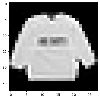

A. torch

# Step1: 데이터정리 (dls생성)
ds = torch.utils.data.TensorDataset(X,y)
dl = torch.utils.data.DataLoader(ds,batch_size=128) 
# Step2: 적합에 필요한 오브젝트 생성
net1 = torch.nn.Sequential(
    torch.nn.Conv2d(1,16,(5,5)),
    torch.nn.ReLU(),
    torch.nn.MaxPool2d((2,2)),
    torch.nn.Flatten()
)
net2 = torch.nn.Sequential(
    torch.nn.Linear(2304,10),
)
net = torch.nn.Sequential(
    net1, # 2d-part
    net2, # 1d-part 
)
loss_fn = torch.nn.CrossEntropyLoss()
optimizr = torch.optim.Adam(net.parameters())
# Step3: 적합 
net.to("cuda:0")
for epoc in range(10):
    for xi,yi in dl:
        ## 1
        ## 2
        loss = loss_fn(net(xi.to("cuda:0")),yi.to("cuda:0"))
        ## 3 
        loss.backward()
        ## 4 
        optimizr.step()
        optimizr.zero_grad()
net.to("cpu")
# Step4: 예측 및 평가 
print(f'train: {(net(X).data.argmax(axis=1) == y).float().mean():.4f}')
print(f'val: {(net(XX).data.argmax(axis=1) == yy).float().mean():.4f}')

train: 0.9077
val: 0.8723

B. fastai

# Step1: 데이터정리 (dls생성)
ds1 = torch.utils.data.TensorDataset(X,y)
ds2 = torch.utils.data.TensorDataset(XX,yy)
dl1 = torch.utils.data.DataLoader(ds1,batch_size=128) 
dl2 = torch.utils.data.DataLoader(ds2,batch_size=100) 
dls = fastai.data.core.DataLoaders(dl1,dl2)
# Step2: 적합에 필요한 오브젝트 생성
net1 = torch.nn.Sequential(
    torch.nn.Conv2d(1,16,(5,5)),
    torch.nn.ReLU(),
    torch.nn.MaxPool2d((2,2)),
    torch.nn.Flatten()
)
net2 = torch.nn.Sequential(
    torch.nn.Linear(2304,10),
)
net = torch.nn.Sequential(
    net1, # 2d-part
    net2, # 1d-part 
)
loss_fn = torch.nn.CrossEntropyLoss()
#optimizr = torch.optim.Adam(net.parameters())
lrnr = fastai.learner.Learner(
    dls=dls,
    model=net,
    loss_func=loss_fn,
    #--#
    metrics=[fastai.metrics.accuracy]
)
# Step3: 적합 
lrnr.fit(10)
# Step4: 예측 및 평가 

lrnr.model.to("cpu")
print(f'train: {(lrnr.model(X).data.argmax(axis=1) == y).float().mean():.4f}')
print(f'val: {(lrnr.model(XX).data.argmax(axis=1) == yy).float().mean():.4f}')

epoch	train_loss	valid_loss	accuracy	time
0	0.484642	0.444805	0.858300	00:01
1	0.393360	0.413498	0.862200	00:01
2	0.340997	0.403366	0.866100	00:01
3	0.310863	0.421401	0.866300	00:01
4	0.291870	0.426586	0.865400	00:01
5	0.277852	0.429622	0.866500	00:01
6	0.266723	0.444076	0.870700	00:01
7	0.260530	0.456487	0.871100	00:01
8	0.253032	0.458816	0.875000	00:01
9	0.247392	0.483315	0.870800	00:01

train: 0.9124
val: 0.8708

6. ImageNet – 직접설계/transfer

A. 알렉스넷(Krizhevsky, Sutskever, and Hinton 2012)의 의미

Krizhevsky, Alex, Ilya Sutskever, and Geoffrey E Hinton. 2012. “Imagenet Classification with Deep Convolutional Neural Networks.” Advances in Neural Information Processing Systems 25.

- 야사로 배우는 인공지능: https://brunch.co.kr/@hvnpoet/109

B. 알렉스넷의 아키텍처 써보기

- 알렉스넷의 아키텍처:

-ref: https://en.wikipedia.org/wiki/AlexNet#:~:text=AlexNet%20is%20the%20name%20of,at%20the%20University%20of%20Toronto.

- 재미삼아 써보면..

img = torch.zeros(1,3*227*227).reshape(1,3,227,227)
img.shape

torch.Size([1, 3, 227, 227])

net = torch.nn.Sequential(
    torch.nn.Conv2d(3,96,kernel_size=(11,11),stride=4),
    torch.nn.ReLU(),    
    torch.nn.MaxPool2d((3,3),stride=2), # default stride는 3
    torch.nn.Conv2d(96,256,kernel_size=(5,5),padding=2),
    torch.nn.ReLU(),
    torch.nn.MaxPool2d((3,3),stride=2), # default stride는 3
    torch.nn.Conv2d(256,384,kernel_size=(3,3),padding=1),
    torch.nn.ReLU(),
    torch.nn.Conv2d(384,384,kernel_size=(3,3),padding=1),
    torch.nn.ReLU(),    
    torch.nn.Conv2d(384,256,kernel_size=(3,3),padding=1),
    torch.nn.ReLU(),    
    torch.nn.MaxPool2d((3,3),stride=2),
    torch.nn.Flatten(),
    torch.nn.Linear(9216,4096),
    torch.nn.ReLU(),
    torch.nn.Dropout(0.5),
    torch.nn.Linear(4096,4096),        
    torch.nn.ReLU(),
    torch.nn.Dropout(0.5),    
    torch.nn.Linear(4096,1000),
)

- 참고사항: torchvision.models.alexnet()을 이용하여 네크워크를 선언할 수도 있음.

torchvision.models.alexnet()

AlexNet(
  (features): Sequential(
    (0): Conv2d(3, 64, kernel_size=(11, 11), stride=(4, 4), padding=(2, 2))
    (1): ReLU(inplace=True)
    (2): MaxPool2d(kernel_size=3, stride=2, padding=0, dilation=1, ceil_mode=False)
    (3): Conv2d(64, 192, kernel_size=(5, 5), stride=(1, 1), padding=(2, 2))
    (4): ReLU(inplace=True)
    (5): MaxPool2d(kernel_size=3, stride=2, padding=0, dilation=1, ceil_mode=False)
    (6): Conv2d(192, 384, kernel_size=(3, 3), stride=(1, 1), padding=(1, 1))
    (7): ReLU(inplace=True)
    (8): Conv2d(384, 256, kernel_size=(3, 3), stride=(1, 1), padding=(1, 1))
    (9): ReLU(inplace=True)
    (10): Conv2d(256, 256, kernel_size=(3, 3), stride=(1, 1), padding=(1, 1))
    (11): ReLU(inplace=True)
    (12): MaxPool2d(kernel_size=3, stride=2, padding=0, dilation=1, ceil_mode=False)
  )
  (avgpool): AdaptiveAvgPool2d(output_size=(6, 6))
  (classifier): Sequential(
    (0): Dropout(p=0.5, inplace=False)
    (1): Linear(in_features=9216, out_features=4096, bias=True)
    (2): ReLU(inplace=True)
    (3): Dropout(p=0.5, inplace=False)
    (4): Linear(in_features=4096, out_features=4096, bias=True)
    (5): ReLU(inplace=True)
    (6): Linear(in_features=4096, out_features=1000, bias=True)
  )
)

Note

직접구현한 알렉스넷과 torchvision.models.alexnet()를 이용한 알렉스넷은 약간다름.

그 이유는 파이토치에서는 원래 논문에서 구현된 알렉스넷이 아니라 이후 수정된 알렉스넷을 사용하기 때문임. 이 내용은 파이토치 공식홈페이지에서 아래와 같이 명시되어있음.

AlexNet was originally introduced in the ImageNet Classification with Deep Convolutional Neural Networks paper. Our implementation is based instead on the “One weird trick” paper above.

ref: https://pytorch.org/vision/main/models/generated/torchvision.models.alexnet.html

C. 알렉스넷으로 ImageNet 적합

pass # 데이터가 너무 커서.. 코랩에서 못할것같아요

7. CIFAR10 – transfer

A. dls 만들자

- X,y를 얻자.

path = fastai.data.external.untar_data(fastai.data.external.URLs.CIFAR)
path.ls()

100.00% [168173568/168168549 00:49<00:00]

(#3) [Path('/root/.fastai/data/cifar10/train'),Path('/root/.fastai/data/cifar10/labels.txt'),Path('/root/.fastai/data/cifar10/test')]

labels = [str(l).split('/')[-1] for l in (path/'train').ls()]
labels

['deer',
 'airplane',
 'ship',
 'dog',
 'automobile',
 'truck',
 'cat',
 'frog',
 'horse',
 'bird']

X = torch.stack([torchvision.io.read_image(str(fname)) for l in labels for fname in (path/f'train/{l}').ls()],axis=0).float()/255
XX = torch.stack([torchvision.io.read_image(str(fname)) for l in labels for fname in (path/f'test/{l}').ls()],axis=0).float()/255
y = torch.tensor([i for i,l in enumerate(labels) for fname in (path/f'train/{l}').ls()])
yy = torch.tensor([i for i,l in enumerate(labels) for fname in (path/f'test/{l}').ls()])

print(X.shape,'\t',X.dtype)
print(y.shape,'\t\t\t',y.dtype)
print(XX.shape,'\t',XX.dtype)
print(yy.shape,'\t\t\t',yy.dtype)

torch.Size([50000, 3, 32, 32])   torch.float32
torch.Size([50000])              torch.int64
torch.Size([10000, 3, 32, 32])   torch.float32
torch.Size([10000])              torch.int64

- 데이터를 시각화해보자.

ylabel = [l for l in labels for fname in (path/f'train/{l}').ls()]
i = 30002
plt.imshow(torch.einsum('cij->ijc',X[i]))
plt.title(f'{ylabel[i]},{y[i]}')

Text(0.5, 1.0, 'cat,6')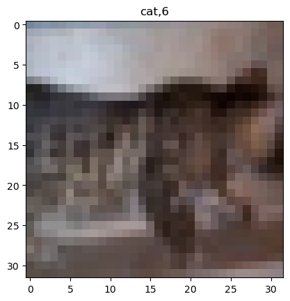

• 그림이 너무 어려운데?
• 맞추기 힘들겠는데..

- dls를 만들자.

ds1 = torch.utils.data.TensorDataset(X,y)
ds2 = torch.utils.data.TensorDataset(XX,yy)
dl1 = torch.utils.data.DataLoader(ds1,batch_size=256,shuffle=True)
dl2 = torch.utils.data.DataLoader(ds2,batch_size=100)
dls = fastai.data.core.DataLoaders(dl1,dl2)

- 아래와 같이 쉽게 만들수도있음…

# dls = fastai.vision.data.ImageDataLoaders.from_folder(path,train='train',valid='test')
# dls.show_batch()

B. 수제네트워크로 학습

- 시도1: 이게 좀 힘들어요 ㅎㅎ

# Step1:
ds1 = torch.utils.data.TensorDataset(X,y)
ds2 = torch.utils.data.TensorDataset(XX,yy)
dl1 = torch.utils.data.DataLoader(ds1,batch_size=256)
dl2 = torch.utils.data.DataLoader(ds2,batch_size=100)
dls = fastai.data.core.DataLoaders(dl1,dl2)
# Step2:
net1 = torch.nn.Sequential(
    torch.nn.Conv2d(3,16,(5,5)),
    torch.nn.ReLU(),
    torch.nn.MaxPool2d((2,2)),
    torch.nn.Flatten()
)
net2 = torch.nn.Sequential(
    torch.nn.Linear(3136,10),
)
net = torch.nn.Sequential(
    net1, # 2d-part
    net2, # 1d-part 
)
loss_fn = torch.nn.CrossEntropyLoss()
lrnr = fastai.learner.Learner(
    dls=dls,
    model=net,
    loss_func=loss_fn,
    #--#
    metrics=[fastai.metrics.accuracy]
)
# Step3:
lrnr.fit(10)
# Step4: 
lrnr.model.to("cpu")
print(f'train: {(lrnr.model(X).data.argmax(axis=1) == y).float().mean():.4f}')
print(f'val: {(lrnr.model(XX).data.argmax(axis=1) == yy).float().mean():.4f}')

epoch	train_loss	valid_loss	accuracy	time
0	2.429019	2.301729	0.121900	00:00
1	2.867480	2.297742	0.121600	00:00
2	2.798708	2.350770	0.099900	00:00
3	2.378768	2.292685	0.116900	00:00
4	2.436424	2.289784	0.126600	00:00
5	2.972414	2.361609	0.122900	00:01
6	2.285441	5.540118	0.100300	00:00
7	2.908635	2.349017	0.131200	00:00
8	3.101591	3.855471	0.103200	00:00
9	2.130486	17.543028	0.100200	00:00

train: 0.1000
val: 0.1002

• ????

- 시도2: 셔플!

# Step1:
ds1 = torch.utils.data.TensorDataset(X,y)
ds2 = torch.utils.data.TensorDataset(XX,yy)
dl1 = torch.utils.data.DataLoader(ds1,batch_size=256,shuffle=True)
dl2 = torch.utils.data.DataLoader(ds2,batch_size=100)
dls = fastai.data.core.DataLoaders(dl1,dl2)
# Step2:
net1 = torch.nn.Sequential(
    torch.nn.Conv2d(3,16,(5,5)),
    torch.nn.ReLU(),
    torch.nn.MaxPool2d((2,2)),
    torch.nn.Flatten()
)
net2 = torch.nn.Sequential(
    torch.nn.Linear(3136,10),
)
net = torch.nn.Sequential(
    net1, # 2d-part
    net2, # 1d-part 
)
loss_fn = torch.nn.CrossEntropyLoss()
lrnr = fastai.learner.Learner(
    dls=dls,
    model=net,
    loss_func=loss_fn,
    #--#
    metrics=[fastai.metrics.accuracy]
)
# Step3:
lrnr.fit(10)
# Step4: 
lrnr.model.to("cpu")
print(f'train: {(lrnr.model(X).data.argmax(axis=1) == y).float().mean():.4f}')
print(f'val: {(lrnr.model(XX).data.argmax(axis=1) == yy).float().mean():.4f}')

epoch	train_loss	valid_loss	accuracy	time
0	1.629887	1.535057	0.463400	00:00
1	1.438346	1.392916	0.512500	00:00
2	1.355882	1.374366	0.518900	00:00
3	1.289650	1.298758	0.542500	00:01
4	1.256436	1.278826	0.555900	00:00
5	1.225732	1.244056	0.563800	00:00
6	1.204093	1.234391	0.563100	00:00
7	1.179638	1.228574	0.569700	00:00
8	1.163272	1.187201	0.585200	00:00
9	1.146735	1.199569	0.578300	00:00

train: 0.6101
val: 0.5783

• 셔플의 차이가 이렇게 크다니??

- 시도3: 복잡하게..

# Step1:
ds1 = torch.utils.data.TensorDataset(X,y)
ds2 = torch.utils.data.TensorDataset(XX,yy)
dl1 = torch.utils.data.DataLoader(ds1,batch_size=256,shuffle=True)
dl2 = torch.utils.data.DataLoader(ds2,batch_size=100)
dls = fastai.data.core.DataLoaders(dl1,dl2)
# Step2:
net1 = torch.nn.Sequential(
    torch.nn.Conv2d(3,256,(5,5)),
    torch.nn.ReLU(),
    torch.nn.Conv2d(256,64,(5,5)),
    torch.nn.ReLU(),
    torch.nn.Conv2d(64,16,(5,5)),
    torch.nn.MaxPool2d((2,2)),
    torch.nn.Flatten()
)
net2 = torch.nn.Sequential(
    torch.nn.Linear(1600,10),
)
net = torch.nn.Sequential(
    net1, # 2d-part
    net2, # 1d-part 
)
loss_fn = torch.nn.CrossEntropyLoss()
lrnr = fastai.learner.Learner(
    dls=dls,
    model=net,
    loss_func=loss_fn,
    #--#
    metrics=[fastai.metrics.accuracy]
)
# Step3:
lrnr.fit(10)
# Step4: 
# 코랩사용시 아래는 주석처리할것 (이유: 코랩의 RAM이 충분하지 않음) valiation set의 accuracy는 fastai결과로 확인할것. 
lrnr.model.to("cpu")
print(f'train: {(lrnr.model(X).data.argmax(axis=1) == y).float().mean():.4f}')
print(f'val: {(lrnr.model(XX).data.argmax(axis=1) == yy).float().mean():.4f}')

epoch	train_loss	valid_loss	accuracy	time
0	1.476197	1.479258	0.465500	00:02
1	1.310572	1.284226	0.538200	00:02
2	1.204503	1.222977	0.572300	00:02
3	1.102717	1.093513	0.615500	00:02
4	1.042015	1.047397	0.627400	00:02
5	0.998049	1.077097	0.621600	00:02
6	0.985487	0.986339	0.660600	00:02
7	0.924648	0.977845	0.663900	00:02
8	0.897980	0.997572	0.658000	00:02
9	0.879995	0.981113	0.660500	00:02

train: 0.7026
val: 0.6605

C. TransferLearning으로 학습

- ResNet18을 다운로드

net = torchvision.models.resnet18()
net

ResNet(
  (conv1): Conv2d(3, 64, kernel_size=(7, 7), stride=(2, 2), padding=(3, 3), bias=False)
  (bn1): BatchNorm2d(64, eps=1e-05, momentum=0.1, affine=True, track_running_stats=True)
  (relu): ReLU(inplace=True)
  (maxpool): MaxPool2d(kernel_size=3, stride=2, padding=1, dilation=1, ceil_mode=False)
  (layer1): Sequential(
    (0): BasicBlock(
      (conv1): Conv2d(64, 64, kernel_size=(3, 3), stride=(1, 1), padding=(1, 1), bias=False)
      (bn1): BatchNorm2d(64, eps=1e-05, momentum=0.1, affine=True, track_running_stats=True)
      (relu): ReLU(inplace=True)
      (conv2): Conv2d(64, 64, kernel_size=(3, 3), stride=(1, 1), padding=(1, 1), bias=False)
      (bn2): BatchNorm2d(64, eps=1e-05, momentum=0.1, affine=True, track_running_stats=True)
    )
    (1): BasicBlock(
      (conv1): Conv2d(64, 64, kernel_size=(3, 3), stride=(1, 1), padding=(1, 1), bias=False)
      (bn1): BatchNorm2d(64, eps=1e-05, momentum=0.1, affine=True, track_running_stats=True)
      (relu): ReLU(inplace=True)
      (conv2): Conv2d(64, 64, kernel_size=(3, 3), stride=(1, 1), padding=(1, 1), bias=False)
      (bn2): BatchNorm2d(64, eps=1e-05, momentum=0.1, affine=True, track_running_stats=True)
    )
  )
  (layer2): Sequential(
    (0): BasicBlock(
      (conv1): Conv2d(64, 128, kernel_size=(3, 3), stride=(2, 2), padding=(1, 1), bias=False)
      (bn1): BatchNorm2d(128, eps=1e-05, momentum=0.1, affine=True, track_running_stats=True)
      (relu): ReLU(inplace=True)
      (conv2): Conv2d(128, 128, kernel_size=(3, 3), stride=(1, 1), padding=(1, 1), bias=False)
      (bn2): BatchNorm2d(128, eps=1e-05, momentum=0.1, affine=True, track_running_stats=True)
      (downsample): Sequential(
        (0): Conv2d(64, 128, kernel_size=(1, 1), stride=(2, 2), bias=False)
        (1): BatchNorm2d(128, eps=1e-05, momentum=0.1, affine=True, track_running_stats=True)
      )
    )
    (1): BasicBlock(
      (conv1): Conv2d(128, 128, kernel_size=(3, 3), stride=(1, 1), padding=(1, 1), bias=False)
      (bn1): BatchNorm2d(128, eps=1e-05, momentum=0.1, affine=True, track_running_stats=True)
      (relu): ReLU(inplace=True)
      (conv2): Conv2d(128, 128, kernel_size=(3, 3), stride=(1, 1), padding=(1, 1), bias=False)
      (bn2): BatchNorm2d(128, eps=1e-05, momentum=0.1, affine=True, track_running_stats=True)
    )
  )
  (layer3): Sequential(
    (0): BasicBlock(
      (conv1): Conv2d(128, 256, kernel_size=(3, 3), stride=(2, 2), padding=(1, 1), bias=False)
      (bn1): BatchNorm2d(256, eps=1e-05, momentum=0.1, affine=True, track_running_stats=True)
      (relu): ReLU(inplace=True)
      (conv2): Conv2d(256, 256, kernel_size=(3, 3), stride=(1, 1), padding=(1, 1), bias=False)
      (bn2): BatchNorm2d(256, eps=1e-05, momentum=0.1, affine=True, track_running_stats=True)
      (downsample): Sequential(
        (0): Conv2d(128, 256, kernel_size=(1, 1), stride=(2, 2), bias=False)
        (1): BatchNorm2d(256, eps=1e-05, momentum=0.1, affine=True, track_running_stats=True)
      )
    )
    (1): BasicBlock(
      (conv1): Conv2d(256, 256, kernel_size=(3, 3), stride=(1, 1), padding=(1, 1), bias=False)
      (bn1): BatchNorm2d(256, eps=1e-05, momentum=0.1, affine=True, track_running_stats=True)
      (relu): ReLU(inplace=True)
      (conv2): Conv2d(256, 256, kernel_size=(3, 3), stride=(1, 1), padding=(1, 1), bias=False)
      (bn2): BatchNorm2d(256, eps=1e-05, momentum=0.1, affine=True, track_running_stats=True)
    )
  )
  (layer4): Sequential(
    (0): BasicBlock(
      (conv1): Conv2d(256, 512, kernel_size=(3, 3), stride=(2, 2), padding=(1, 1), bias=False)
      (bn1): BatchNorm2d(512, eps=1e-05, momentum=0.1, affine=True, track_running_stats=True)
      (relu): ReLU(inplace=True)
      (conv2): Conv2d(512, 512, kernel_size=(3, 3), stride=(1, 1), padding=(1, 1), bias=False)
      (bn2): BatchNorm2d(512, eps=1e-05, momentum=0.1, affine=True, track_running_stats=True)
      (downsample): Sequential(
        (0): Conv2d(256, 512, kernel_size=(1, 1), stride=(2, 2), bias=False)
        (1): BatchNorm2d(512, eps=1e-05, momentum=0.1, affine=True, track_running_stats=True)
      )
    )
    (1): BasicBlock(
      (conv1): Conv2d(512, 512, kernel_size=(3, 3), stride=(1, 1), padding=(1, 1), bias=False)
      (bn1): BatchNorm2d(512, eps=1e-05, momentum=0.1, affine=True, track_running_stats=True)
      (relu): ReLU(inplace=True)
      (conv2): Conv2d(512, 512, kernel_size=(3, 3), stride=(1, 1), padding=(1, 1), bias=False)
      (bn2): BatchNorm2d(512, eps=1e-05, momentum=0.1, affine=True, track_running_stats=True)
    )
  )
  (avgpool): AdaptiveAvgPool2d(output_size=(1, 1))
  (fc): Linear(in_features=512, out_features=1000, bias=True)
)

- 마지막의 레이어만 수정

net.fc = torch.nn.Linear(512,10)

- 학습해보자.

# Step1:
ds1 = torch.utils.data.TensorDataset(X,y)
ds2 = torch.utils.data.TensorDataset(XX,yy)
dl1 = torch.utils.data.DataLoader(ds1,batch_size=64,shuffle=True)
dl2 = torch.utils.data.DataLoader(ds2,batch_size=100)
dls = fastai.data.core.DataLoaders(dl1,dl2)
# Step2:
net = torchvision.models.resnet18()
net.fc = torch.nn.Linear(512,10)
loss_fn = torch.nn.CrossEntropyLoss()
lrnr = fastai.learner.Learner(
    dls=dls,
    model=net,
    loss_func=loss_fn,
    #--#
    metrics=[fastai.metrics.accuracy]
)
# Step3:
lrnr.fit(10)
# Step4: 
# 코랩사용시 아래는 주석처리할것 (이유: 코랩의 RAM이 충분하지 않음) valiation set의 accuracy는 fastai결과로 확인할것. 
lrnr.model.to("cpu")
print(f'train: {(lrnr.model(X).data.argmax(axis=1) == y).float().mean():.4f}') # 
print(f'val: {(lrnr.model(XX).data.argmax(axis=1) == yy).float().mean():.4f}')

epoch	train_loss	valid_loss	accuracy	time
0	1.157889	1.281547	0.540200	00:11
1	0.924410	1.179057	0.596200	00:11
2	0.797667	0.948804	0.678700	00:11
3	0.681159	0.877607	0.699700	00:11
4	0.568150	0.818889	0.726400	00:11
5	0.509804	0.842927	0.725800	00:11
6	0.428966	0.836546	0.736100	00:11
7	0.378433	0.825805	0.753200	00:11
8	0.297282	0.917828	0.734000	00:11
9	0.244396	0.876090	0.763200	00:11

train: 0.9523
val: 0.7632

Caution

통계학과서버를 이용하시는 분들은 다른 학생들을 위하여 실습이 끝난이후 커널을 죽여주시기 바랍니다. 그렇지 않으면 GPU메모리 부족으로 다른학생들이 실습하기 어렵습니다.(무슨말인지 모르겠으면 저에게 물어보세요)

8. HW

없어요..