03wk-2: 깊은 신경망 (1) – 로지스틱의 한계 극복

Author

최규빈

Published

March 20, 2024

1. 강의영상

2. Imports

import torch
import matplotlib.pyplot as plt 
import pandas as pd

3. 꺽인그래프를 만드는 방법

- 로지스틱의 한계를 극복하기 위해서는 시그모이드를 취하기 전에 꺽인 그래프 모양을 만드는 기술이 있어야겠음.

- 아래와 같은 벡터 \({\boldsymbol x}\)를 가정하자.

x = torch.linspace(-1,1,1001).reshape(-1,1)
x

tensor([[-1.0000],
        [-0.9980],
        [-0.9960],
        ...,
        [ 0.9960],
        [ 0.9980],
        [ 1.0000]])

- 목표: 아래와 같은 벡터 \({\boldsymbol y}\)를 만들어보자.

\[{\boldsymbol y} = [y_1,y_2,\dots,y_{n}], \quad y_i = \begin{cases} 9x_i +4.5& x_i <0 \\ -4.5x_i + 4.5& x_i >0 \end{cases}\]

A. 방법1

y = x*0 
y[x<0] = (9*x+4.5)[x<0]
y[x>0] = (-4.5*x+4.5)[x>0]

plt.plot(y,'--')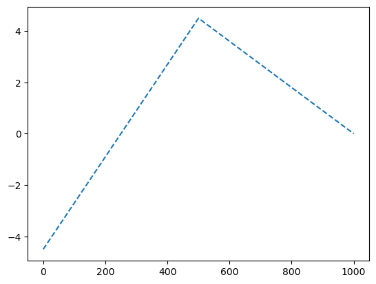

Note

강의영상에 보셨듯이 아래의 코드실행결과는 다르게 나옵니다.

## 아래를 실행하면 꺽인선이 나오는데용...
x = torch.linspace(-1,1,1001).reshape(-1,1)
y = x*0 + x 
y[x<0] = (9*x+4.5)[x<0]
y[x>0] = (-4.5*x+4.5)[x>0]
plt.plot(x,y)

## 이걸 실행하면 그냥 직선이 나옵니다...
x = torch.linspace(-1,1,1001).reshape(-1,1)
y = x 
y[x<0] = (9*x+4.5)[x<0]
y[x>0] = (-4.5*x+4.5)[x>0]
plt.plot(x,y)

다르게 나오는 이유가 너무 궁금하시다면 아래의 링크로 가셔서 깊은복사/얕은복사에 대한 개념을 이해하시면 됩니다. (그렇지만 가능하다면 궁금해하지 마세요…..)

깊은복사 얕은복사 강의들으러 가기

B. 방법2 – 렐루이용

relu = torch.nn.ReLU()

plt.plot(relu(x),'--',label=r'$relu(x)$')
plt.plot(relu(-x),'--',label=r'$relu(-x)$')
plt.legend()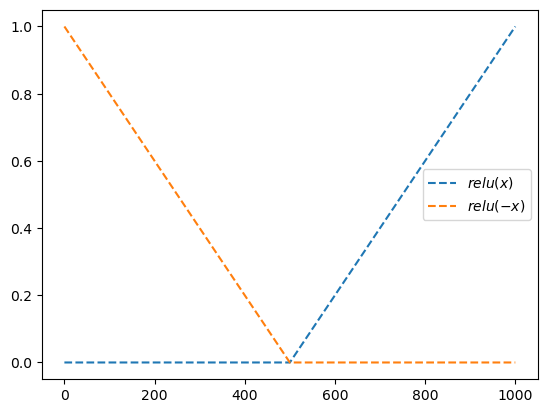

plt.plot(-4.5*relu(x),'--',label=r'$-4.5\times relu(x) + 4.5$')
plt.plot(-9*relu(-x),'--',label=r'$-9\times relu(-x) + 4.5$')
plt.legend()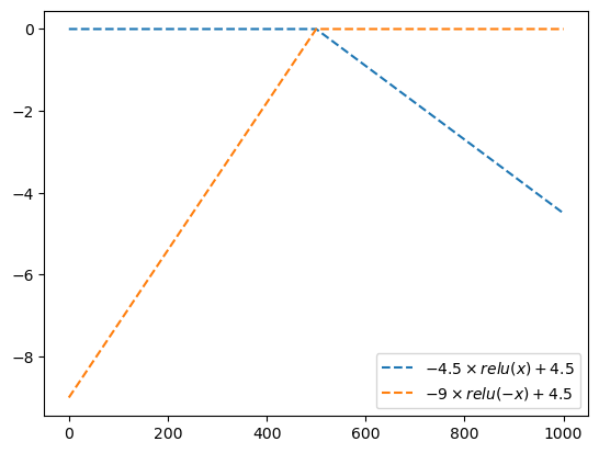

plt.plot(-4.5*relu(x)-9*relu(-x),'--',label=r'$-4.5\times relu(x) -9 \times relu(-x)$')
plt.plot(y,'--',label=r'$y$')
plt.plot(-4.5*relu(x)-9*relu(-x)+4.5,'--',label=r'$-4.5\times relu(x) -9 \times relu(-x)+4.5$')
plt.legend()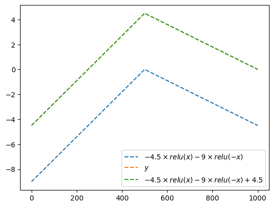

- 우리의 목표: 저 초록선에서 시그모이드를 태우면된다. 즉 아래의 느낌임

sig = torch.nn.Sigmoid()

fig = plt.figure(figsize=(8, 4))
spec = fig.add_gridspec(4, 4)
ax1 = fig.add_subplot(spec[:2,0]); ax1.set_title(r'$x$'); ax1.set_ylim(-1,1)
ax2 = fig.add_subplot(spec[2:,0]); ax2.set_title(r'$-x$'); ax2.set_ylim(-1,1)
ax3 = fig.add_subplot(spec[:2,1]); ax3.set_title(r'$relu(x)$'); ax3.set_ylim(-1,1)
ax4 = fig.add_subplot(spec[2:,1]); ax4.set_title(r'$relu(-x)$'); ax4.set_ylim(-1,1)
ax5 = fig.add_subplot(spec[1:3,2]); ax5.set_title(r'$-4.5 relu(x)-9 relu(-x)+4.5$')
ax6 = fig.add_subplot(spec[1:3,3]); ax6.set_title('sig(...)');
#---#
ax1.plot(x,'--',color='C0')
ax2.plot(-x,'--',color='C1')
ax3.plot(relu(x),'--',color='C0')
ax4.plot(relu(-x),'--',color='C1')
ax5.plot(-4.5*relu(x)-9*relu(-x)+4.5,'--',color='C2')
ax6.plot(sig(-4.5*relu(x)-9*relu(-x)+4.5),'--',color='C2')
fig.tight_layout()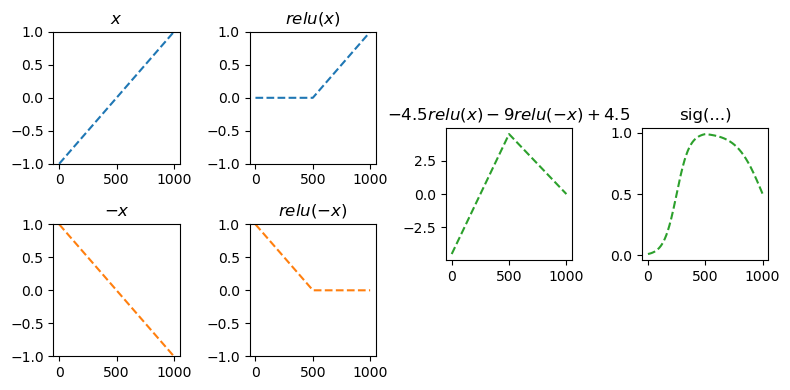

C. 방법2의 다른구현

- 렐루이용하여 만드는 방법 정리

벡터 x와 relu함수를 준비한다.
u = [x,-x] 를 계산한다.
v = [relu(x), relu(-x)] 를 계산한다.
y = -4.5 * relu(x) + 9 * relu(-x) +4.5 를 계산한다.

- 1단계

x,relu

(tensor([[-1.0000],
         [-0.9980],
         [-0.9960],
         ...,
         [ 0.9960],
         [ 0.9980],
         [ 1.0000]]),
 ReLU())

- 2단계

u = torch.concat([x,-x],axis=1) # u = [x, -x] 같은것
u

tensor([[-1.0000,  1.0000],
        [-0.9980,  0.9980],
        [-0.9960,  0.9960],
        ...,
        [ 0.9960, -0.9960],
        [ 0.9980, -0.9980],
        [ 1.0000, -1.0000]])

- 3단계

v = relu(u) # 각각의 column에 렐루취함
v

tensor([[0.0000, 1.0000],
        [0.0000, 0.9980],
        [0.0000, 0.9960],
        ...,
        [0.9960, 0.0000],
        [0.9980, 0.0000],
        [1.0000, 0.0000]])

- 4단계

-4.5 * v[:,[0]] - 9.0 * v[:,[1]] +4.5

tensor([[-4.5000],
        [-4.4820],
        [-4.4640],
        ...,
        [ 0.0180],
        [ 0.0090],
        [ 0.0000]])

tensor([[-4.5000],
        [-4.4820],
        [-4.4640],
        ...,
        [ 0.0180],
        [ 0.0090],
        [ 0.0000]])

- 그런데, 4단계는 아래와 같이 볼 수 있다.

\({\boldsymbol v}\begin{bmatrix} -4.5 \\ -9.0 \end{bmatrix} + 4.5 = \begin{bmatrix} v_{11} & v_{12} \\ v_{21} & v_{22} \\ \dots & \dots \\ v_{n1} & v_{n2} \\ \end{bmatrix}\begin{bmatrix} -4.5 \\ -9.0 \end{bmatrix} + 4.5 = \begin{bmatrix} -4.5 v_{11} - 9.0 v_{12} + 4.5 \\ -4.5 v_{21} - 9.0 v_{22} + 4.5 \\ \dots \\ -4.5 v_{n1} - 9.0 v_{n2} + 4.5 \\ \end{bmatrix}\)

위의 수식을 참고하여 매트릭스의 곱 형태로 다시 포현하면 아래와 같다.

#-4.5 * v[:,[0]] - 9.0 * v[:,[1]] +4.5
What = torch.tensor([[-4.5],[-9.0]]) 
v @ What + 4.5

tensor([[-4.5000],
        [-4.4820],
        [-4.4640],
        ...,
        [ 0.0180],
        [ 0.0090],
        [ 0.0000]])

이제 매트릭스의 곱 대신에 torch.nn.Linear()를 이용하면 아래의 코드와 같아진다.

l2 = torch.nn.Linear(
    in_features=2,
    out_features=1 
)

l2.weight.data = torch.tensor([[-4.5,-9.0]])
l2.bias.data = torch.tensor([4.5])

l2(v)

tensor([[-4.5000],
        [-4.4820],
        [-4.4640],
        ...,
        [ 0.0180],
        [ 0.0090],
        [ 0.0000]], grad_fn=<AddmmBackward0>)

- 사실 2단계도 아래와 같이 볼 수 있다.

\[\begin{bmatrix} x_1 \\ x_2 \\ \dots \\ x_n \end{bmatrix}\begin{bmatrix} 1 & -1 \end{bmatrix} = \begin{bmatrix} x_1 & -x_1 \\ x_2 & -x_2 \\ \dots & \dots \\ x_n & -x_n \end{bmatrix}\]

#u = torch.concat([x,-x],axis=1) # u1 = [x, -x] 같은것

l1 = torch.nn.Linear(1,2)
l1.weight.data = torch.tensor([[1.0],[-1.0]])
l1.bias.data = torch.tensor([0.0,0.0])

l1(x)

tensor([[-1.0000,  1.0000],
        [-0.9980,  0.9980],
        [-0.9960,  0.9960],
        ...,
        [ 0.9960, -0.9960],
        [ 0.9980, -0.9980],
        [ 1.0000, -1.0000]], grad_fn=<AddmmBackward0>)

- 따라서 torch.nn 에 포함된 레이어를 이용하면 아래와 같이 표현할 할 수 있다.

l1 = torch.nn.Linear(1,2)
l1.weight.data = torch.tensor([[1.0],[-1.0]])
l1.bias.data = torch.tensor([0.0,0.0])
a1 = torch.nn.ReLU()
l2 = torch.nn.Linear(2,1)
l2.weight.data = torch.tensor([[-4.5,-9.0]])
l2.bias.data = torch.tensor([4.5])

l2(a1(l1(x))), y

(tensor([[-4.5000],
         [-4.4820],
         [-4.4640],
         ...,
         [ 0.0180],
         [ 0.0090],
         [ 0.0000]], grad_fn=<AddmmBackward0>),
 tensor([[-4.5000],
         [-4.4820],
         [-4.4640],
         ...,
         [ 0.0180],
         [ 0.0090],
         [ 0.0000]]))

- 각각의 layer를 torch.nn.Sequential() 로 묶으면 아래와 같이 정리할 수 있다.

net = torch.nn.Sequential(
    torch.nn.Linear(1,2),
    torch.nn.ReLU(),
    torch.nn.Linear(2,1)
)
l1,a1,l2 = net
l1.weight.data = torch.tensor([[1.0],[-1.0]])
l1.bias.data = torch.tensor([0.0,0.0])
l2.weight.data = torch.tensor([[-4.5,-9.0]])
l2.bias.data = torch.tensor([4.5])

net(x),y

(tensor([[-4.5000],
         [-4.4820],
         [-4.4640],
         ...,
         [ 0.0180],
         [ 0.0090],
         [ 0.0000]], grad_fn=<AddmmBackward0>),
 tensor([[-4.5000],
         [-4.4820],
         [-4.4640],
         ...,
         [ 0.0180],
         [ 0.0090],
         [ 0.0000]]))

D. 수식표현

(1) \({\bf X}=\begin{bmatrix} x_1 \\ \dots \\ x_n \end{bmatrix}\)

(2) \(l_1({\bf X})={\bf X}{\bf W}^{(1)}\overset{bc}{+} {\boldsymbol b}^{(1)}=\begin{bmatrix} x_1 & -x_1 \\ x_2 & -x_2 \\ \dots & \dots \\ x_n & -x_n\end{bmatrix}\)

\({\bf W}^{(1)}=\begin{bmatrix} 1 & -1 \end{bmatrix}\)
\({\boldsymbol b}^{(1)}=\begin{bmatrix} 0 & 0 \end{bmatrix}\)

(3) \((a_1\circ l_1)({\bf X})=\text{relu}\big({\bf X}{\bf W}^{(1)}\overset{bc}{+}{\boldsymbol b}^{(1)}\big)=\begin{bmatrix} \text{relu}(x_1) & \text{relu}(-x_1) \\ \text{relu}(x_2) & \text{relu}(-x_2) \\ \dots & \dots \\ \text{relu}(x_n) & \text{relu}(-x_n)\end{bmatrix}\)

(4) \((l_2 \circ a_1\circ l_1)({\bf X})=\text{relu}\big({\bf X}{\bf W}^{(1)}\overset{bc}{+}{\boldsymbol b}^{(1)}\big){\bf W}^{(2)}\overset{bc}{+}b^{(2)}\)

\(\quad=\begin{bmatrix} -4.5\times\text{relu}(x_1) -9.0 \times \text{relu}(-x_1) +4.5 \\ -4.5\times\text{relu}(x_2) -9.0 \times\text{relu}(-x_2) + 4.5 \\ \dots \\ -4.5\times \text{relu}(x_n) -9.0 \times\text{relu}(-x_n)+4.5 \end{bmatrix}\)

\({\bf W}^{(2)}=\begin{bmatrix} -4.5 \\ -9 \end{bmatrix}\)
\(b^{(2)}=4.5\)

(5) \(net({\bf X})=(l_2 \circ a_1\circ l_1)({\bf X})=\text{relu}\big({\bf X}{\bf W}^{(1)}\overset{bc}{+}{\boldsymbol b}^{(1)}\big){\bf W}^{(2)}\overset{bc}{+}b^{(2)}\)

\(\quad =\begin{bmatrix} -4.5\times\text{relu}(x_1) -9.0 \times \text{relu}(-x_1) +4.5 \\ -4.5\times\text{relu}(x_2) -9.0 \times\text{relu}(-x_2) + 4.5 \\ \dots \\ -4.5\times \text{relu}(x_n) -9.0 \times\text{relu}(-x_n)+4.5 \end{bmatrix}\)

4. 로지스틱의 한계 극복

A. 데이터

df = pd.read_csv("https://raw.githubusercontent.com/guebin/DL2024/main/posts/dnnex.csv")
df

	x	prob	y
0	-1.000000	0.000045	0.0
1	-0.998999	0.000046	0.0
2	-0.997999	0.000047	0.0
3	-0.996998	0.000047	0.0
4	-0.995998	0.000048	0.0
...	...	...	...
1995	0.995998	0.505002	0.0
1996	0.996998	0.503752	0.0
1997	0.997999	0.502501	0.0
1998	0.998999	0.501251	1.0
1999	1.000000	0.500000	1.0

2000 rows × 3 columns

x = torch.tensor(df.x).float().reshape(-1,1)
y = torch.tensor(df.y).float().reshape(-1,1)
prob = torch.tensor(df.prob).float().reshape(-1,1)

plt.plot(x,y,'o',alpha=0.02)
plt.plot(x[0],y[0],'o',label= r"observed data = $(x_i,y_i)$",color="C0")
plt.plot(x,prob,'--b',label= r"prob (true, unknown)")
plt.legend()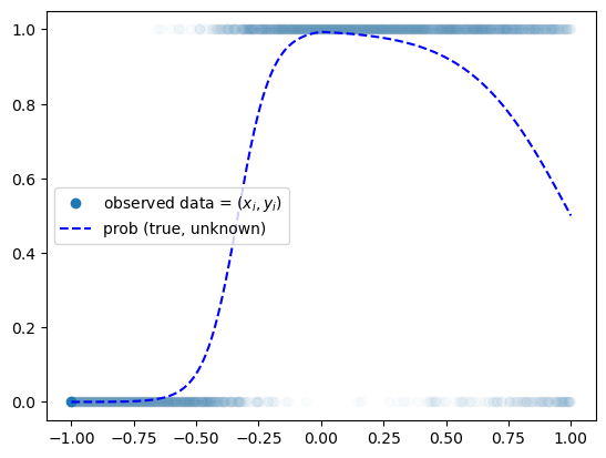

B. Step 1~4

- Step1에 대한 생각: 네트워크를 어떻게 만들까? = 아키텍처를 어떻게 만들까? = 모델링

\[\underset{(n,1)}{\bf X} \overset{l_1}{\to} \underset{(n,2)}{\boldsymbol u^{(1)}} \overset{a_1}{\to} \underset{(n,2)}{\boldsymbol v^{(1)}} \overset{l_1}{\to} \underset{(n,1)}{\boldsymbol u^{(2)}} \overset{a_2}{\to} \underset{(n,1)}{\boldsymbol v^{(2)}}=\underset{(n,1)}{\hat{\boldsymbol y}}\]

- Step2,3,4 는 너무 뻔해서..

torch.manual_seed(43052)
net = torch.nn.Sequential(
    torch.nn.Linear(1,2),
    torch.nn.ReLU(),
    torch.nn.Linear(2,1),
    torch.nn.Sigmoid()
)
loss_fn = torch.nn.BCELoss()
optimizr = torch.optim.Adam(net.parameters())
#---#
for epoc in range(3000):
    ## 
    yhat = net(x)
    ## 
    loss = loss_fn(yhat,y)
    ## 
    loss.backward()
    ## 
    optimizr.step()
    optimizr.zero_grad()

plt.plot(x,y,'o',alpha=0.02)
plt.plot(x[0],y[0],'o',label= r"observed data = $(x_i,y_i)$",color="C0")
plt.plot(x,prob,'--b',label= r"prob (true, unknown)")
plt.plot(x,net(x).data,'--',label="prob (estimated) -- after 3000 epochs")
plt.legend()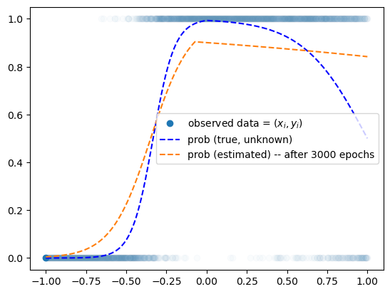

for epoc in range(3000):
    ## 
    yhat = net(x)
    ## 
    loss = loss_fn(yhat,y)
    ## 
    loss.backward()
    ## 
    optimizr.step()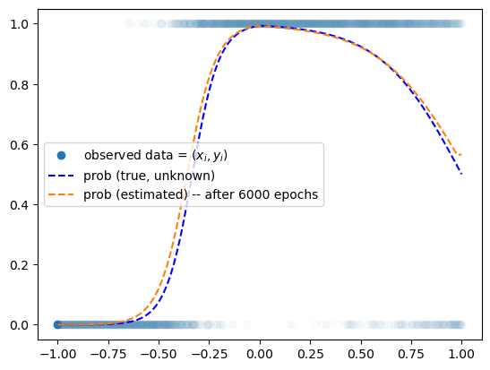
    optimizr.zero_grad()

plt.plot(x,y,'o',alpha=0.02)
plt.plot(x[0],y[0],'o',label= r"observed data = $(x_i,y_i)$",color="C0")
plt.plot(x,prob,'--b',label= r"prob (true, unknown)")
plt.plot(x,net(x).data,'--',label="prob (estimated) -- after 6000 epochs")
plt.legend()