02wk-1: 회귀분석 (2) – Step1~4 / 벡터미분

1. 강의영상

2. Imports

import torch
import matplotlib.pyplot as plt 
import numpy as np

3. 회귀모형

A. 소설

- 카페주인인 박혜원씨는 온도와 아이스아메리카노 판매량이 관계가 있다는 것을 알았다. 구체적으로는

“온도가 높아질 수록 (=날씨가 더울수록) 아이스아메리카노의 판매량이 증가”

한다는 사실을 알게 되었다. 박혜원씨는

일기예보를 보고 오늘의 평균 기온을 입력하면, 오늘의 아이스아메리카노 판매량을 미리 예측할 수 있지 않을까? 그 예측량만큼 아이스아메리카노를 준비하면 장사에 도움이 되지 않을까???

라는 생각을 하게 되었고 이를 위하여 아래와 같이 100개의 데이터를 모았다.

temp = [-2.4821, -2.3621, -1.9973, -1.6239, -1.4792, -1.4635, -1.4509, -1.4435,
        -1.3722, -1.3079, -1.1904, -1.1092, -1.1054, -1.0875, -0.9469, -0.9319,
        -0.8643, -0.7858, -0.7549, -0.7421, -0.6948, -0.6103, -0.5830, -0.5621,
        -0.5506, -0.5058, -0.4806, -0.4738, -0.4710, -0.4676, -0.3874, -0.3719,
        -0.3688, -0.3159, -0.2775, -0.2772, -0.2734, -0.2721, -0.2668, -0.2155,
        -0.2000, -0.1816, -0.1708, -0.1565, -0.1448, -0.1361, -0.1057, -0.0603,
        -0.0559, -0.0214,  0.0655,  0.0684,  0.1195,  0.1420,  0.1521,  0.1568,
         0.2646,  0.2656,  0.3157,  0.3220,  0.3461,  0.3984,  0.4190,  0.5443,
         0.5579,  0.5913,  0.6148,  0.6469,  0.6469,  0.6523,  0.6674,  0.7059,
         0.7141,  0.7822,  0.8154,  0.8668,  0.9291,  0.9804,  0.9853,  0.9941,
         1.0376,  1.0393,  1.0697,  1.1024,  1.1126,  1.1532,  1.2289,  1.3403,
         1.3494,  1.4279,  1.4994,  1.5031,  1.5437,  1.6789,  2.0832,  2.2444,
         2.3935,  2.6056,  2.6057,  2.6632]

sales= [-8.5420, -6.5767, -5.9496, -4.4794, -4.2516, -3.1326, -4.0239, -4.1862,
        -3.3403, -2.2027, -2.0262, -2.5619, -1.3353, -2.0466, -0.4664, -1.3513,
        -1.6472, -0.1089, -0.3071, -0.6299, -0.0438,  0.4163,  0.4166, -0.0943,
         0.2662,  0.4591,  0.8905,  0.8998,  0.6314,  1.3845,  0.8085,  1.2594,
         1.1211,  1.9232,  1.0619,  1.3552,  2.1161,  1.1437,  1.6245,  1.7639,
         1.6022,  1.7465,  0.9830,  1.7824,  2.1116,  2.8621,  2.1165,  1.5226,
         2.5572,  2.8361,  3.3956,  2.0679,  2.8140,  3.4852,  3.6059,  2.5966,
         2.8854,  3.9173,  3.6527,  4.1029,  4.3125,  3.4026,  3.2180,  4.5686,
         4.3772,  4.3075,  4.4895,  4.4827,  5.3170,  5.4987,  5.4632,  6.0328,
         5.2842,  5.0539,  5.4538,  6.0337,  5.7250,  5.7587,  6.2020,  6.5992,
         6.4621,  6.5140,  6.6846,  7.3497,  8.0909,  7.0794,  6.8667,  7.4229,
         7.2544,  7.1967,  9.5006,  9.0339,  7.4887,  9.0759, 11.0946, 10.3260,
        12.2665, 13.0983, 12.5468, 13.8340]

여기에서 temp는 평균기온이고, sales는 아이스아메리카노 판매량이다.¹ 평균기온과 판매량의 그래프를 그려보면 아래와 같다.

¹ 판매량이 소수점이고 심지어 음수인것은 그냥 그려러니 하자..

plt.plot(temp,sales,'o')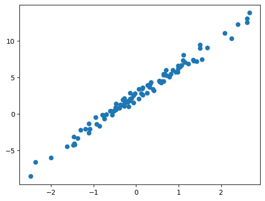

B. 모델링

- 산점도를 살펴본 박혜원씨는 평균기온이 올라갈수록 아이스아메리카노 판매량이 “선형적”으로 증가한다는 사실을 캐치했다. 물론 약간의 오차는 있어보였다. 오차까지 고려하여 평균기온과 아이스판매량의 관계를 추정하면 아래와 같이 생각할 수 있다.

아이스아메리카노 판매량 \(\approx\) \(w_0\) \(+\) \(w_1\) \(\times\) 평균기온

위의 수식에서 만약에 \(w_0\)와 \(w_1\)의 값을 적절히 추정한다면, 평균기온량을 입력으로 하였을때 아이스아메리카노 판매량을 예측할 수 있을 것이다.

- 아이스크림 판매량을 \(y_i\)로, 평균기온을 \(x_i\)로 변수화한뒤 박혜원의 수식을 좀 더 수학적으로 표현하면

\[y_i \approx w_0 + w_1 x_i,\quad i=1,2,\dots,100\]

와 같이 쓸 수 있다. 오차항을 포함하여 좀 더 엄밀하게 쓰면

\[y_i = w_0 + w_1 x_i + \epsilon_i,\quad i=1,2,\dots,100\]

와 같이 나타낼 수 있어보인다. 여기에서 \(\epsilon_i \sim N(0,\sigma^2)\) 로 가정해도 무방할 듯 하다. 그런데 이를 다시 아래와 같이 표현하는 것이 가능하다.

\[{\bf y}={\bf X}{\bf W} +\boldsymbol{\epsilon}\]

단 여기에서

\[{\bf y}=\begin{bmatrix} y_1 \\ y_2 \\ \dots \\ y_n\end{bmatrix}, \quad {\bf x}=\begin{bmatrix} x_1 \\ x_2 \\ \dots \\ x_n\end{bmatrix}, \quad {\bf X}=\begin{bmatrix} {\bf 1} & {\bf x} \end{bmatrix}=\begin{bmatrix} 1 & x_1 \\ 1 & x_2 \\ \dots \\ 1 & x_n\end{bmatrix}, \quad {\bf W}=\begin{bmatrix} w_0 \\ w_1 \end{bmatrix}, \quad \boldsymbol{\epsilon}= \begin{bmatrix} \epsilon_1 \\ \dots \\ \epsilon_n\end{bmatrix}\]

이다.

C. 데이터를 torch.tensor로 변환

- 현재까지의 상황을 파이토치로 코딩하면 아래와 같다.

x = torch.tensor(temp).reshape(-1,1)
ones = torch.ones(100).reshape(-1,1)
X = torch.concat([ones,x],axis=1)
y = torch.tensor(sales).reshape(-1,1)
#W = ?? 이건 모름.. 추정해야함. 
#ϵ = ?? 이것도 모름!!

D. 아무렇게나 추정

- \({\bf W}\) 에 대한 추정값을 \(\hat{\bf W}\)라고 할때

\[\hat{\bf W}=\begin{bmatrix} \hat{w}_0 \\ \hat{w}_1 \end{bmatrix} =\begin{bmatrix} -5 \\ 10 \end{bmatrix}\]

으로 추정한 상황이라면 커피판매량의 예측값은

\[\hat{\bf y} = {\bf X}\hat{\bf W}\]

이라고 표현할 수 있다. 이 의미는 아래의 그림에서 주황색 점선으로 커피판매량을 예측한다는 의미이다.

What = torch.tensor([[-5.0],
                     [10.0]])
What

tensor([[-5.],
        [10.]])

yhat = X@What

plt.plot(x,y,'o')
plt.plot(x,yhat,'--')

E. 추정의 방법

- 방법1: 이론적으로 추론 <- 회귀분석시간에 배운것

torch.linalg.inv((X.T @ X)) @ X.T @ y # 공식~

tensor([[2.4459],
        [4.0043]])

plt.plot(x,y,'o')
plt.plot(x,2.4459 + 4.0043*x,'--')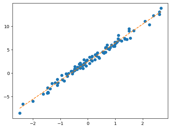

- 방법2: 컴퓨터의 반복계산을 이용하여 추론 (손실함수도입 + 경사하강법)

• 1단계: 아무 점선이나 그어본다..
• 2단계: 1단계에서 그은 점선보다 더 좋은 점선으로 바꾼다.
• 3단계: 1-2단계를 반복한다.

4. 파이토치의 반복추정

A. 문제셋팅 다시 복습

x = torch.tensor(temp).reshape(-1,1)
ones = torch.ones(100).reshape(-1,1)
X = torch.concat([ones,x],axis=1)
y = torch.tensor(sales).reshape(-1,1)

B. 1단계 – 최초의 점선

What = torch.tensor([[-5.0],[10.0]],requires_grad=True)
What

tensor([[-5.],
        [10.]], requires_grad=True)

yhat = X@What 

plt.plot(x,y,'o')
plt.plot(x,yhat.data,'--') # 그림을 그리기 위해서 yhat의 미분꼬리표를 제거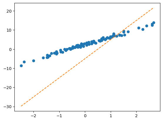

C. 2단계 – update

- ’적당한 정도’를 판단하기 위한 장치: loss function 도입!

\[loss=\sum_{i=1}^{n}(y_i-\hat{y}_i)^2=\sum_{i=1}^{n}(y_i-(\hat{w}_0+\hat{w}_1x_i))^2=({\bf y}-{\bf\hat{y}})^\top({\bf y}-{\bf\hat{y}})=({\bf y}-{\bf X}{\bf \hat{W}})^\top({\bf y}-{\bf X}{\bf \hat{W}})\]

- loss 함수의 특징

• \(y_i \approx \hat{y}_i\) 일수록 loss값이 작다.
• \(y_i \approx \hat{y}_i\) 이 되도록 \((\hat{w}_0,\hat{w}_1)\)을 잘 찍으면 loss값이 작다.
• (중요) 주황색 점선이 ‘적당할 수록’ loss값이 작다.

loss = torch.sum((y-yhat)**2)
loss

tensor(8587.6240, grad_fn=<SumBackward0>)

- 우리의 목표: 이 loss(=8587.6240)을 더 줄이자.

• 궁극적으로는 아예 모든 조합 \((\hat{w}_0,\hat{w}_1)\)에 대하여 가장 작은 loss를 찾으면 좋겠다.

- 발상의 전환: 가만히 보니까 loss는 \(\hat{\bf W} =\begin{bmatrix} \hat{w}_0 \\ \hat{w}_1 \end{bmatrix}\) 에 따라서 값이 바뀌는 함수잖아??? 즉 아래와 같이 생각할 수 있음.

\[ loss(\hat{w}_0,\hat{w}_1) := loss(\hat{\bf W})=\sum_{i=1}^{n}(y_i-(\hat{w}_0+\hat{w}_1x_i))^2=({\bf y}-{\bf X}{\bf \hat{W}})^\top({\bf y}-{\bf X}{\bf \hat{W}})\]

따라서 구하고 싶은것은 아래와 같음

\[\hat{\bf W} := \underset{\bf W}{\operatorname{argmin}} ~ loss({\bf W})\]

- \(loss({\bf W})\)를 최소로 만드는 \({\bf W}\)를 컴퓨터로 구하는 방법, 즉 \(\hat{\bf W} := \underset{\bf W}{\operatorname{argmin}} ~ loss({\bf W})\)를 구하는 방법을 요약하면 아래와 같다.

1. 임의의 점 \(\hat{\bf W}\)를 찍는다.

2. 그 점에서 순간기울기를 구한다. 즉 \(\frac{\partial}{\partial {\bf W}}loss({\bf W})\) 를 계산한다.

3. \(\hat{\bf W}\)에서의 순간기울기²의 부호를 살펴보고 부호와 반대방향으로 움직인다. 이때 기울기의 절대값 크기³와 비례하여 보폭(=움직이는 정도)을 각각 조절한다. 즉 아래의 수식에 따라 업데이트 한다.

² \(\frac{\partial}{\partial {\bf W}}loss({\bf W})\)

³ \(\left|\frac{\partial}{\partial {\bf W}}loss({\bf W})\right|\)

\[\hat{\bf W} \leftarrow \hat{\bf W} - \alpha \times \frac{\partial}{\partial {\bf W}}loss({\bf W})\]

- 여기에서 미분을 어떻게…?? 즉 아래를 어떻게 계산해..?

\[\frac{\partial}{\partial {\bf W}}loss({\bf W}):= \begin{bmatrix} \frac{\partial}{\partial w_0} \\ \frac{\partial}{\partial w_1}\end{bmatrix}loss({\bf W}) = \begin{bmatrix} \frac{\partial}{\partial w_0}loss({\bf W}) \\ \frac{\partial}{\partial w_1}loss({\bf W})\end{bmatrix} \]

loss.backward()를 실행하면 What.grad에 미분값이 업데이트 되어요!

(실행전)

print(What.grad)

None

(실행후)

loss.backward()

print(What.grad)

tensor([[-1342.2465],
        [ 1188.9203]])

- 계산결과의 검토 (1)

• \(loss({\bf W})=({\bf y}-\hat{\bf y})^\top ({\bf y}-\hat{\bf y})=({\bf y}-{\bf XW})^\top ({\bf y}-{\bf XW})\)

• \(\frac{\partial}{\partial {\bf W}}loss({\bf W})=-2{\bf X}^\top {\bf y}+2{\bf X}^\top {\bf X W}\)

- 2 * X.T @ y + 2 * X.T @ X @ What

tensor([[-1342.2466],
        [ 1188.9198]], grad_fn=<AddBackward0>)

- 계산결과의 검토 (2)

\[\frac{\partial}{\partial {\bf W} } loss({\bf W})=\begin{bmatrix}\frac{\partial}{\partial w_0} \\ \frac{\partial}{\partial w_1} \end{bmatrix}loss({\bf W}) =\begin{bmatrix}\frac{\partial}{\partial w_0}loss(w_0,w_1) \\ \frac{\partial}{\partial w_1}loss(w_0,w_1) \end{bmatrix}\]

를 계산하고 싶은데 벡터미분을 할줄 모른다고 하자. 편미분의 정의를 살펴보면,

\[\frac{\partial}{\partial w_0}loss(w_0,w_1) \approx \frac{loss(w_0+h,w_1)-loss(w_0,w_1)}{h}\]

\[\frac{\partial}{\partial w_1}loss(w_0,w_1) \approx \frac{loss(w_0,w_1+h)-loss(w_0,w_1)}{h}\]

라고 볼 수 있다. 이를 이용하여 근사계산하면

def l(w0,w1):
    return torch.sum((y-w0-w1*x)**2)

l(-5,10), loss # 로스값일치

(tensor(8587.6240), tensor(8587.6240, grad_fn=<SumBackward0>))

h=0.001 
(l(-5+h,10) - l(-5,10))/h

tensor(-1342.7733)

h=0.001 
(l(-5,10+h) - l(-5,10))/h

tensor(1189.4531)

이 값은 What.grad에 저장된 값과 거의 비슷하다.

What.grad

tensor([[-1342.2465],
        [ 1188.9203]])

- 이제 아래의 공식에 넣고 업데이트해보자

\[\hat{\bf W} \leftarrow \hat{\bf W} - \alpha \times \frac{\partial}{\partial {\bf W}}loss({\bf W})\]

alpha = 0.001 
print(f"{What.data} -- 수정전")
print(f"{-alpha*What.grad} -- 수정하는폭")
print(f"{What.data-alpha*What.grad} -- 수정후")
print(f"{torch.linalg.inv((X.T @ X)) @ X.T @ y} -- 회귀분석으로 구한값")
print(f"{torch.tensor([[2.5],[4]])} -- 참값(이건 비밀~~)")

tensor([[-5.],
        [10.]]) -- 수정전
tensor([[ 1.3422],
        [-1.1889]]) -- 수정하는폭
tensor([[-3.6578],
        [ 8.8111]]) -- 수정후
tensor([[2.4459],
        [4.0043]]) -- 회귀분석으로 구한값
tensor([[2.5000],
        [4.0000]]) -- 참값(이건 비밀~~)

• alpha를 잘 잡아야함~

- 1회 수정결과를 시각화

Wbefore = What.data
Wafter = What.data - alpha * What.grad 
Wbefore, Wafter

(tensor([[-5.],
         [10.]]),
 tensor([[-3.6578],
         [ 8.8111]]))

plt.plot(x,y,'o',label=r'observed data')
plt.plot(x,X@Wbefore,'--', label=r"$\hat{\bf y}_{before}={\bf X}@\hat{\bf W}_{before}$")
plt.plot(x,X@Wafter,'--', label=r"$\hat{\bf y}_{after}={\bf X}@\hat{\bf W}_{after}$")
plt.legend()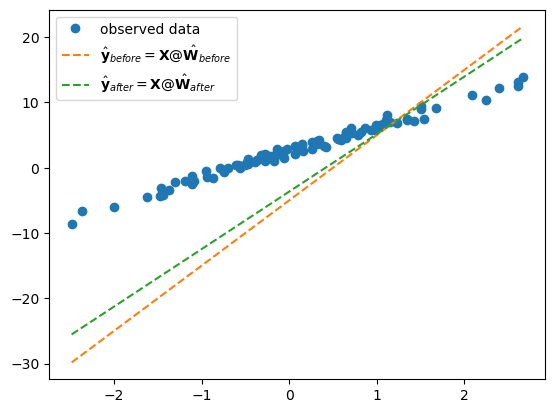

D. 3단계 – iteration (=learn = estimate \(\bf{\hat W}\))

x = torch.tensor(temp).reshape(-1,1)
ones = torch.ones(100).reshape(-1,1)
X = torch.concat([ones,x],axis=1)
y = torch.tensor(sales).reshape(-1,1)

What = torch.tensor([[-5.0],[10.0]],requires_grad=True)
What

tensor([[-5.],
        [10.]], requires_grad=True)

for epoc in range(30):
    yhat = X @ What
    loss = torch.sum((y-yhat)**2)
    loss.backward()
    What.data = What.data - 0.001 * What.grad
    What.grad = None

plt.plot(x,y,'o', label = "ovserved data")
plt.plot(x,X@What.data,'--', label = r"$\hat{\bf y}={\bf X}@\hat{\bf W}$ after 30 iterations (=epochs)")
plt.legend()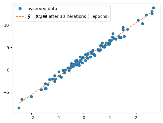

5. 파라메터의 학습과정 음미

A. 단순무식한 print

What = torch.tensor([[-5.0],[10.0]],requires_grad=True)
alpha = 0.001
print(f"시작값 = {What.data.reshape(-1)}")
for epoc in range(30):
    yhat = X @ What
    loss = torch.sum((y-yhat)**2)
    loss.backward()
    What.data = What.data - 0.001 * What.grad
    print(f'loss = {loss:.2f} \t 업데이트폭 = {-0.001 * What.grad.reshape(-1)} \t 업데이트결과: {What.data.reshape(-1)}')
    What.grad = None

시작값 = tensor([-5., 10.])
loss = 8587.62   업데이트폭 = tensor([ 1.3422, -1.1889])      업데이트결과: tensor([-3.6578,  8.8111])
loss = 5675.18   업데이트폭 = tensor([ 1.1029, -0.9499])      업데이트결과: tensor([-2.5548,  7.8612])
loss = 3755.63   업데이트폭 = tensor([ 0.9056, -0.7596])      업데이트결과: tensor([-1.6492,  7.1016])
loss = 2489.58   업데이트폭 = tensor([ 0.7431, -0.6081])      업데이트결과: tensor([-0.9061,  6.4935])
loss = 1654.04   업데이트폭 = tensor([ 0.6094, -0.4872])      업데이트결과: tensor([-0.2967,  6.0063])
loss = 1102.33   업데이트폭 = tensor([ 0.4995, -0.3907])      업데이트결과: tensor([0.2028, 5.6156])
loss = 737.85    업데이트폭 = tensor([ 0.4091, -0.3136])      업데이트결과: tensor([0.6119, 5.3020])
loss = 496.97    업데이트폭 = tensor([ 0.3350, -0.2519])      업데이트결과: tensor([0.9469, 5.0501])
loss = 337.72    업데이트폭 = tensor([ 0.2742, -0.2025])      업데이트결과: tensor([1.2211, 4.8477])
loss = 232.40    업데이트폭 = tensor([ 0.2243, -0.1629])      업데이트결과: tensor([1.4453, 4.6848])
loss = 162.73    업데이트폭 = tensor([ 0.1834, -0.1311])      업데이트결과: tensor([1.6288, 4.5537])
loss = 116.64    업데이트폭 = tensor([ 0.1500, -0.1056])      업데이트결과: tensor([1.7787, 4.4481])
loss = 86.13     업데이트폭 = tensor([ 0.1226, -0.0851])      업데이트결과: tensor([1.9013, 4.3629])
loss = 65.94     업데이트폭 = tensor([ 0.1001, -0.0687])      업데이트결과: tensor([2.0014, 4.2942])
loss = 52.57     업데이트폭 = tensor([ 0.0818, -0.0554])      업데이트결과: tensor([2.0832, 4.2388])
loss = 43.72     업데이트폭 = tensor([ 0.0668, -0.0447])      업데이트결과: tensor([2.1500, 4.1941])
loss = 37.86     업데이트폭 = tensor([ 0.0545, -0.0361])      업데이트결과: tensor([2.2045, 4.1579])
loss = 33.98     업데이트폭 = tensor([ 0.0445, -0.0292])      업데이트결과: tensor([2.2490, 4.1287])
loss = 31.41     업데이트폭 = tensor([ 0.0363, -0.0236])      업데이트결과: tensor([2.2853, 4.1051])
loss = 29.70     업데이트폭 = tensor([ 0.0296, -0.0191])      업데이트결과: tensor([2.3150, 4.0860])
loss = 28.58     업데이트폭 = tensor([ 0.0242, -0.0155])      업데이트결과: tensor([2.3391, 4.0705])
loss = 27.83     업데이트폭 = tensor([ 0.0197, -0.0125])      업데이트결과: tensor([2.3589, 4.0580])
loss = 27.33     업데이트폭 = tensor([ 0.0161, -0.0101])      업데이트결과: tensor([2.3749, 4.0479])
loss = 27.01     업데이트폭 = tensor([ 0.0131, -0.0082])      업데이트결과: tensor([2.3881, 4.0396])
loss = 26.79     업데이트폭 = tensor([ 0.0107, -0.0067])      업데이트결과: tensor([2.3988, 4.0330])
loss = 26.65     업데이트폭 = tensor([ 0.0087, -0.0054])      업데이트결과: tensor([2.4075, 4.0276])
loss = 26.55     업데이트폭 = tensor([ 0.0071, -0.0044])      업데이트결과: tensor([2.4146, 4.0232])
loss = 26.49     업데이트폭 = tensor([ 0.0058, -0.0035])      업데이트결과: tensor([2.4204, 4.0197])
loss = 26.45     업데이트폭 = tensor([ 0.0047, -0.0029])      업데이트결과: tensor([2.4251, 4.0168])
loss = 26.42     업데이트폭 = tensor([ 0.0038, -0.0023])      업데이트결과: tensor([2.4289, 4.0145])

B. 반복시각화 – yhat의 관점에서!

What = torch.tensor([[-5.0],[10.0]],requires_grad=True)
alpha = 0.001
fig = plt.plot(x,y,'o',label = "observed")
plt.plot(x,X@What.data,'--',color="C1")
for epoc in range(30):
    yhat = X @ What
    loss = torch.sum((y-yhat)**2)
    loss.backward()
    What.data = What.data - 0.001 * What.grad
    plt.plot(x,X@What.data,'--',color="C1",alpha=0.1)
    What.grad = None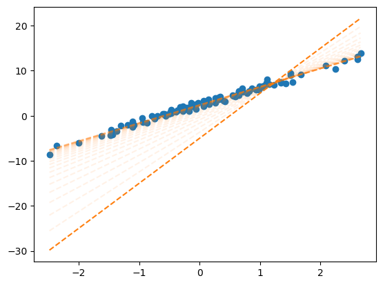

C. 반복시각화 – loss의 관점에서!!

def plot_loss():
    fig = plt.figure()
    ax = fig.add_subplot(projection='3d')
    w0 = np.arange(-6, 11, 0.5) 
    w1 = np.arange(-6, 11, 0.5)
    W1,W0 = np.meshgrid(w1,w0)
    LOSS=W0*0
    for i in range(len(w0)):
        for j in range(len(w1)):
            LOSS[i,j]=torch.sum((y-w0[i]-w1[j]*x)**2)
    ax.plot_surface(W0, W1, LOSS, rstride=1, cstride=1, color='b',alpha=0.1)
    ax.azim = 30  ## 3d plot의 view 조절 
    ax.dist = 8   ## 3d plot의 view 조절 
    ax.elev = 5   ## 3d plot의 view 조절 
    ax.set_xlabel(r'$w_0$')  # x축 레이블 설정
    ax.set_ylabel(r'$w_1$')  # y축 레이블 설정
    ax.set_xticks([-5,0,5,10])  # x축 틱 간격 설정
    ax.set_yticks([-5,0,5,10])  # y축 틱 간격 설정
    return fig

l(-5,10)

tensor(8587.6240)

fig = plot_loss()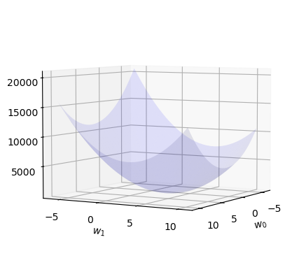

fig = plot_loss()
ax = fig.gca()
ax.scatter(2.5, 4, l(2.5,4), s=200, marker='*', color='red', label=r"${\bf W}=[2.5, 4]'$")
ax.scatter(-5, 10, l(-5,10), s=200, marker='*', color='blue', label=r"initial $\hat{\bf W}=[-5, 10]'$")
ax.legend()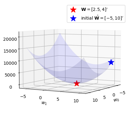

w0,w1 = What.data.reshape(-1)

What.data

tensor([[2.4289],
        [4.0145]])

w0,w1

(tensor(2.4289), tensor(4.0145))

What = torch.tensor([[-5.0],[10.0]],requires_grad=True)
alpha = 0.001
for epoc in range(30):
    yhat = X @ What
    loss = torch.sum((y-yhat)**2)
    loss.backward()
    What.data = What.data - 0.001 * What.grad
    w0,w1 = What.data.reshape(-1) 
    ax.scatter(w0,w1,l(w0,w1),s=5,marker='o',color='blue')
    What.grad = None

fig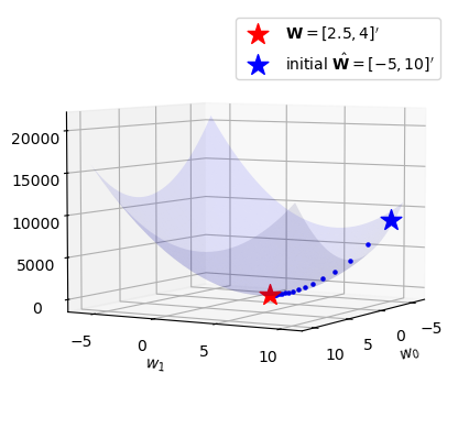

D. 애니메이션

from matplotlib import animation

plt.rcParams['figure.figsize'] = (7.5,2.5)
plt.rcParams["animation.html"] = "jshtml" 

def show_animation(alpha=0.001):
    ## 1. 히스토리 기록을 위한 list 초기화
    loss_history = [] 
    yhat_history = [] 
    What_history = [] 

    ## 2. 학습 + 학습과정기록
    What= torch.tensor([[-5.0],[10.0]],requires_grad=True)
    What_history.append(What.data.tolist())
    for epoc in range(30): 
        yhat=X@What ; yhat_history.append(yhat.data.tolist())
        loss=torch.sum((y-yhat)**2); loss_history.append(loss.item())
        loss.backward() 
        What.data = What.data - alpha * What.grad; What_history.append(What.data.tolist())
        What.grad = None    

    ## 3. 시각화 
    fig = plt.figure()
    ax1 = fig.add_subplot(1, 2, 1)
    ax2 = fig.add_subplot(1, 2, 2, projection='3d')

    #### ax1: yhat의 관점에서.. 
    ax1.plot(x,y,'o',label=r"$(x_i,y_i)$")
    line, = ax1.plot(x,yhat_history[0],label=r"$(x_i,\hat{y}_i)$") 
    ax1.legend()
    #### ax2: loss의 관점에서.. 
    w0 = np.arange(-6, 11, 0.5) 
    w1 = np.arange(-6, 11, 0.5)
    W1,W0 = np.meshgrid(w1,w0)
    LOSS=W0*0
    for i in range(len(w0)):
        for j in range(len(w1)):
            LOSS[i,j]=torch.sum((y-w0[i]-w1[j]*x)**2)
    ax2.plot_surface(W0, W1, LOSS, rstride=1, cstride=1, color='b',alpha=0.1)
    ax2.azim = 30  ## 3d plot의 view 조절 
    ax2.dist = 8   ## 3d plot의 view 조절 
    ax2.elev = 5   ## 3d plot의 view 조절 
    ax2.set_xlabel(r'$w_0$')  # x축 레이블 설정
    ax2.set_ylabel(r'$w_1$')  # y축 레이블 설정
    ax2.set_xticks([-5,0,5,10])  # x축 틱 간격 설정
    ax2.set_yticks([-5,0,5,10])  # y축 틱 간격 설정
    ax2.scatter(2.5, 4, l(2.5,4), s=200, marker='*', color='red', label=r"${\bf W}=[2.5, 4]'$")
    ax2.scatter(-5, 10, l(-5,10), s=200, marker='*', color='blue')
    ax2.legend()
    def animate(epoc):
        line.set_ydata(yhat_history[epoc])
        ax2.scatter(np.array(What_history)[epoc,0],np.array(What_history)[epoc,1],loss_history[epoc],color='grey')
        fig.suptitle(f"alpha = {alpha} / epoch = {epoc}")
        return line

    ani = animation.FuncAnimation(fig, animate, frames=30)
    plt.close()
    return ani

epoch = 0 부터 시작하여 시작점에서 출발하도록 애니메이션을 수정했습니당.

ani = show_animation(alpha=0.001)
ani

Once Loop Reflect

E. 학습률에 따른 시각화

- \(\alpha\)가 너무 작다면 비효율적임

show_animation(alpha=0.0001)

Once Loop Reflect

- \(\alpha\)가 크다고 무조건 좋은건 또 아님

show_animation(alpha=0.0083)

Once Loop Reflect

- 수틀리면 수렴안할수도??

show_animation(alpha=0.0085)

Once Loop Reflect

- 그냥 망할수도??

show_animation(alpha=0.01)

Once Loop Reflect

6. HW

학습률\((\alpha\))를 조정하면서 실습해보고 스크린샷 제출

A1. 벡터미분

A. 해결하고 싶은것

아래와 같은 선형모형이 있다고 가정하자.

\[{\bf y}={\bf X}{\boldsymbol \beta} + {\boldsymbol \epsilon}\]

이러한 모형에 대하여 아래와 같이 손실함수를 정의하자.

\[loss({\boldsymbol \beta}) = ({\bf y} - {\bf X}{\boldsymbol \beta})^\top({\bf y} - {\bf X}{\boldsymbol \beta}) \]

이때 손실함수의 미분값을 아래와 같이 주어지고,

\[\frac{\partial}{\partial {\boldsymbol \beta}}loss({\boldsymbol \beta}) = -2{\bf X}^\top{\bf y}+2{\bf X}^\top{\bf X}{\boldsymbol \beta}\]

따라서 손실함수를 최소화하는 추정량이 아래와 같이 주어짐을 보여라.

\[\hat{\boldsymbol \beta} = ({\bf X}^\top {\bf X})^{-1}{\bf X}^\top{\bf y}\]

B. 해설강의 및 보충자료

https://github.com/guebin/DL2024/blob/main/posts/02wksupp.pdf